How to Use a Data Validation Formula When Creating a Budget

Use Formulas in Data Validation

Use a Formula in Data Validation

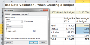
Recently, one of my viewers wanted to know which formula he could use to prevent an end-user from imputing a value that would exceed his budget. I created this video tutorial to demonstrate my response.

Use a Formula in Data Validation

I have identified Data Validation as one of the “Nine Essential Skills in Excel.” Here is one example – Using a Formula in Data Validation to prevent an input entry from exceeding a set budget amount

A Formula that Evaluates to TRUE

The “key” to understanding how use Formulas in Data Validation – When the formula answer is TRUE, the entry is accepted; When the answer to the formula is FALSE, the Error Message that you create prevents an invalid entry.

Remember, that in Data Validation, only the STOP style will prevent an invalid entry.!

Video Training Resources

9 Essential Skills for Excel 2010

9 Essential Skills for Excel 2010 Video Tutorial

I invite you to visit my secure online shopping website – http://shop.thecompanyrocks.com – to preview the many video training resources that I offer you.

Watch This Tutorial in High Definition

Follow this link to watch my Excel Tutorial in High Definition on my YouTube Channel – DannyRocksExcels

Share and Enjoy:
  • Add to favorites
  • Facebook
  • Twitter
  • Technorati
  • Print
  • email
  • Digg
  • StumbleUpon
  • del.icio.us
  • Yahoo! Buzz
  • Google Bookmarks
  • Orkut
  • SphereIt
  • Sphinn

Essential Excel Skill #3: Creating and Using Named Cell Ranges in Excel

Essential Skill #3 - Using Named Cell Ranges

Essential Excel Skill 33 – Using Named Cell Ranges

I believe that there are two main reasons to create and use Named Cell Ranges in Excel”

  • They make great Navigational Bookmarks – to quickly move to a specific location in your workbook
  • Using Named Cell Ranges in Excel Formulas make the formula:
    • Easier to Write
    • Easier to Explain – to others
    • Easier to Understand – when you need to edit it or copy it.

9 Essential Excel Skills

My latest Excel Video Training Resource: “9 Essential Excel Skills,” contains 4 hours of focused video training. There are a total of 25 individual video tutorials in the resource.

Here, in this lesson, I demonstrate several of the tips and techniques that I present in Essential Skill # 3. I show you how easy it is to create and use Named Cell Ranges in Excel Formulas and Functions.

Secure Online Shopping at The Company Rocks

I invite you to visit my secure, online shopping website – http://shop.thecompanyrocks.com – to explore all of the training resources that I offer you.

Watch My Tutorial in High Definition

Follow this link to watch my Excel tutorial in High Definition on my YouTube Channel – DannyRocksExcels

Share and Enjoy:
  • Add to favorites
  • Facebook
  • Twitter
  • Technorati
  • Print
  • email
  • Digg
  • StumbleUpon
  • del.icio.us
  • Yahoo! Buzz
  • Google Bookmarks
  • Orkut
  • SphereIt
  • Sphinn

Two Glowing Reviews for my Excel Video Tutorials

Today, two of my customers posted glowing reviews for my Excel Video Tutorials. Thank you! Thank you! Thank you!

9 Essential Skills for Excel 2010

9 Essential Skills for Excel 2010 Video Tutorial

“Nine Essential Skills for Excel 2010”

“In my opinion the 9 Essential Skills for Excel 2010 , is an outstanding training video. It covers a lot of the required intermediate requirements. One thing that really stands out for me is the method of presentation. Danny always:

  • a) explains what he is going to do in simple languageĀ 
  • b)demonstrates what he has just explained
  • c)shows you where to find the icons on the ribbon
  • d)shows you the keyboard shortcuts to use(they actually appear on the video as they are used.

The video also had a good introduction to the value of using tables. Like all of Danny’s videos this should be a fantastic success.

– John J, Canada

Pivot Tables for Excel 2003

“Excel 2003 Pivot Tables to Summarize, Analyze, and Present Information”

“A mere few hours with your Excel 2003 course and I was able to
perform pivot table operations which had eluded me for over a year
using multiple other publications totaling nearly 1,500 pages: while those sources are terrific, each of us learns differently, your courses certainly fill that learning gap for me.

I deal with mostly with cumulative metrics, that is, incremental, week to week.

After two evenings of your course, I was able to build tables presenting the year, month, quarter & weekly totals of the multiple tools deployed, and, amazingly, display the incremental changes down to a week-to-week basis.

You had mentioned that you hoped I enjoyed the course, of course, I enjoyed the course – indeed, but after a year-plus struggle with several other sources, the *learning* from your course was the true reward!”

– Paul B., Colorado

Learn More About My Video Training Resources

I am confident that you will learn many valuable tips and techniques from my extended length Excel Video Training Resources.My Motto is:

“I work hard to make it easy for you to get the most out of Microsoft Excel”

Follow these links to learn more about my video training resources:

Share and Enjoy:
  • Add to favorites
  • Facebook
  • Twitter
  • Technorati
  • Print
  • email
  • Digg
  • StumbleUpon
  • del.icio.us
  • Yahoo! Buzz
  • Google Bookmarks
  • Orkut
  • SphereIt
  • Sphinn

The 10 Most Watched Excel YouTube Videos for September 2012

My YouTube Channel – DannyRocksExcels – had 141,586 individual views during the month of September 2012:

Here is a list – with Hyperlinks – to the 10 Most Watched Excel Videos

Top 10 YouTube Excel Videos

  1. Compare Two Excel Lists to Spot the Differences– 5,304 views in September
    1. Go to this Blog Post on my website
  2. How to Merge Multiple Excel Workbooks to a Master Budget – 4,915 views in September
    1. Go to this Blog Post on my website
  3. How to Use Advanced Filters in Excel– 4,660 views in September
    1. Go to this Blog Post on my website
  4. How to Add a Check Box Control to an Excel Form– 4,301 views in September
    1. Go to this Blog Post on my website
  5. Use the Built-in Data Form in Excel to View and Filter Records– 3,948 views in September
    1. Go to this Blog Post on my website
  6. How to Create a Summary Report from an Excel Table-3,932 views in September
    1. Go to this Blog Post on my website
  7. How to Create an Interactive Excel Pivot Chart– 3,696 views in September
    1. Go to this Blog Post on my website
  8. Consolidating Data from Multiple Excel Worksheets by Position– 3,618 views in September
    1. Go to this Blog Post on my website
  9. How to Use the Solver Tool in Excel– 3,532 views in September
    1. Go to this Blog Post on my website
  10. How to Use an Excel Data Table for “What-if” Analysis– 3,513 views in September
    1. Go to this Blog Post on my website

Thanks to my 4,500 Subscriber on YouTube!

I extend my heartfelt thanks to my many loyal viewers and subscribers to my Excel video tutorials. Your feedback and requests for solutions have formed the foundation for my Excel Training Videos.

9 Essential Excel 2010 Skills

9 Essential Excel 2010 Skills

Learn More About my Extended Length Excel Video Training Resources

I have created a series of Extended Length Video Training Resources in the category of “Master Excel in Minutes.” I invite you to follow this link to learn more about my new series of videos.

Share and Enjoy:
  • Add to favorites
  • Facebook
  • Twitter
  • Technorati
  • Print
  • email
  • Digg
  • StumbleUpon
  • del.icio.us
  • Yahoo! Buzz
  • Google Bookmarks
  • Orkut
  • SphereIt
  • Sphinn

Instructional Guide “9 Essential Excel 2010 Skills” – Download for Free

Instructional Guide "9 Essential Excel 2010 Skills"

Instructional Guide “9 Essential Excel 2010 Skills”

I want you to discover the scope of the Excel Training that I offer on my new video tutorial, “9 Essential Excel 2010 Skills.” So, I am offering the PDF of the Step-by-Step Instructional Guide that accompanies the video tutorial.

Link to The Company Rocks Free Resources Page

Click on this link to begin the download process for the Instructional Guide.

Instructions for Downloading the Free Instructional Guide

  1. Add this product to your secure shopping cart at my website.
  2. During Checkout, you can choose to either Register or Shop as a Guest
  3. You will need to provide a valid email address in order to receive the actual link to download my Instructional Guide.
  4. Even though you will be downloading this product, I had to set it up as a physical product with “Free Shipping.”
  5. Shortly after you complete the checkout process you will receive an email that contains a hyperlink to the file that you will download.
  6. You will be downloading a “zipped” file. So, once the download is completed, be sure to “unzip” this file!
  7. I created my Instructional Guide using the free Adobe Acrobat Reader.

Read the Instructional Guide and then Purchase my Video!

I am convinced that once you see the scope of the training in Excel 2010 that I offer, you will want to purchase the video tutorial. I offer my video in tow versions:

List of the “9 Essential Excel 2010 Skills”

9 Essential Skills for Excel 2010

9 Essential Skills for Excel 2010 Video Tutorial

These are the 9 Essential Skills that I have identified for my video tutorial:

  1. Entering Data Efficiently in Excel 2010
  2. Selecting Cell Ranges Efficiently in Excel 2010
  3. Creating and Using Named Cell Ranges in Excel 2010
  4. Applying Styles and Formatting to Excel 2010 Worksheets
  5. Working with Structured Data Sets in Excel 2010
  6. Working with Excel 2010 Formulas and Functions
  7. Using Paste Special Options in Excel 2010
  8. Using Data Validation in Excel 2010
  9. Using Excel 2010 “What-if” Analysis Tools

Excel 2010 Practice Files Included

When you purchase my video tutorial, you receive the same Excel 2010 Worksheets that I used while filming each of the 25 video tutorials. Using the same files as you view my videos, you will be able to practice your new skills. And, of course, you also receive the same Instructional Guide that I am offering for free!

I welcome your feedback! Please send me your comments via email – danny@thecompanyrocks.com – or by adding a comment below.

Thank you!


Share and Enjoy:
  • Add to favorites
  • Facebook
  • Twitter
  • Technorati
  • Print
  • email
  • Digg
  • StumbleUpon
  • del.icio.us
  • Yahoo! Buzz
  • Google Bookmarks
  • Orkut
  • SphereIt
  • Sphinn

How to Dynamically Color-Code Dates with Conditional Formatting in Excel

Conditional Formatting for Dates

Conditional Formatting for Dates

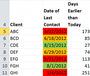
One of my viewers wants to learn how to “dynamically” color-code cells that contain dates. She is monitoring the frequency of contact with her clients and she wants Excel to automatically apply:

  • One background color to cells where it has been less than 60 days since last contact
  • A different color when the time frame is between 60 and 90 days
  • A third color when it has been over 90 days since the last contact with a client

Here, I demonstrate how she can do this using Conditional Formatting Rules. However, this will only work if you are using Excel 2007 or Excel 2010.

Understanding Dynamic Date Functions

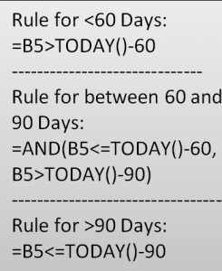
In order to make this visualization “dynamic,” I make references to cells that contain the =TODAY() Function. This is a “volatile” function that updates automatically based upon the date in your computer system’s clock. I use this to classify the last date of contact with her clients.

Improvements in Conditional Formatting

Beginning with Excel 2007, you can now apply multiple rules that use formulas. Remember that when you use a formula, it must evaluate as “TRUE” in order to apply the formatting that you specify.

Formulas Used to Apply Conditional Formatting

Conditional Formatting Rules

Rules for Conditional Formatting

To make it easier for you to practice this skill, I have posted this table that details the formulas that I used for each of the three rules in my video tutorial.Note that with the middle condition, I use the =AND() Function. All logical tests must answer TRUE for the AND() Function to return TRUE.

It will take a little bit of practice for you to become comfortable with these formulas. As a Best Practice, I recommend that you create a table of formulas so that you can see how a “tweak” in your formula can turn a FALSE answer into a TRUE answer.

Related Video

Follow this link to Part Two in this Series. I demonstrate how to “toggle” Conditional Formatting On or Off by using a Check Box Control in Excel.

Watch this Video in High Definition

Follow this link to watch my Excel Tutorial in High Definition on my YouTube Channel – DannyRocksExcels

Get the Best Tips and Training for Excel

Click on this link to learn more about my best-selling DVD-ROM, “The 50 Best Tips for Excel 2007.” This link will take you to my secure online shopping website –Ā  http://shop.thecompanyrocks.com

Subscribe to my Video Podcast on iTunes

Here is the link to go to my free Video Podcast, “Danny Rocks Tips and Timesavers” on iTunes.


Share and Enjoy:
  • Add to favorites
  • Facebook
  • Twitter
  • Technorati
  • Print
  • email
  • Digg
  • StumbleUpon
  • del.icio.us
  • Yahoo! Buzz
  • Google Bookmarks
  • Orkut
  • SphereIt
  • Sphinn

How to Place Dates in a Fiscal Year Quarter

Many organizations operate in a Fiscal Year – for example, April 1 through March 31 of the next calendar year. I get many requests from viewers for help with placing calendar dates into the proper Quarter for their Fiscal Year.

Excel Functions Used in Video TutorialWhile researching a question from one viewer, I cam across a very interesting formula that nests the “undocumented” DATEDIF() Function inside the CEILING() Function. I found this formula in the book, “Formulas and Functions with MS Excel 2003,” written by Paul McFedries. It is a very efficient formula.

What is Covered on the Video

Watch this video tutorial as I break down each step. As a Best Practice, I recommend that you break down a complex formula by working from the “inside out.” I start with the “nested” DATEDIF() function and then demonstrate the results of each formula detail.

Learn More About the “Undocumented” DATEDIF() Function

For various reasons, Microsoft does not offer any help or documentation for the very useful DATEDIF() Function. In fact, it is not even listed as a Function! However, it is very useful and often found in VBA (Visual Basic for Applications) coding. Here, are links to two videos that I created to help you understand how to use DATEDIF():

Learn How to Calculate a Calendar Year Quarter

In response to viewer requests, I created a companion video tutorial -” How to Calculate a Calendar Year Quarter in Excel.”

Resources Available at The Company Rocks

I invite you to visit my secure online shopping website – http://shop.thecompanyrocks.com – to preview the many resources that I offer for helping you to improve your software skills.

Watch Video Tutorial in High Definition

If you would like to watch my video tutorial for “Finding the Fiscal Year Quarter for any Date,” click on this link. I have posted it on my YouTube Channel – DannyRocksExcels

Watch this Video Now


Share and Enjoy:
  • Add to favorites
  • Facebook
  • Twitter
  • Technorati
  • Print
  • email
  • Digg
  • StumbleUpon
  • del.icio.us
  • Yahoo! Buzz
  • Google Bookmarks
  • Orkut
  • SphereIt
  • Sphinn

How to Protect Cells that Hold Formulas in Excel

Protect Cells w Formulas

Protect Excel Formula Cells

Learning how to Protect the Excel Worksheet Cells that contain Formulas is a three-step process. This process tends to confuse and frustrate many Excel users. Some of the steps seem counter-intuitive when you first begin the process. That is why I created this video tutorial – To demonstrate each of the steps; to remove the confusion.

First, I show you how this is done in Excel 2010 / Excel 2007. Next, I show you how to protect the Formula Cells in Excel 2003.

Key Concept for Protecting Formula Cells

By default, all cells in an Excel Workbook are “Locked!”

So, if you are going to allow a user to input current values in the worksheet, you must first “select” the input cells and then, “Unlock” them.

Protecting Excel Worksheet

The final step in the process is to Protect the Worksheet. I rarely use a password for the worksheet because I tend to forget it and then I cannot even access the protected worksheet!

Take care in the Protect Sheet Dialog Box to select only the options that best suit your purpose. For example, in this video tutorial, I choose to limit users to select only the cells that I unlocked in steps 1 and 2.

Go To Special Dialog Box

The quickest way to select the cells that you wish to “unlock” is to open the Go To Special Dialog Box. There, choose “Constants.” You can limit the constants to “Numbers” as I do in this tutorial.

Danny Rocks Tips and Timesavers Podcast on iTunes

I invite you to subscribe to my “free” video podcast on iTunes. Click on this link to access all of my Podcast Videos.

Watch Tutorial in High Definition

Follow this link to view this Excel Tutorial in High Definition on my YouTube Channel – DannyRocksExcels


Share and Enjoy:
  • Add to favorites
  • Facebook
  • Twitter
  • Technorati
  • Print
  • email
  • Digg
  • StumbleUpon
  • del.icio.us
  • Yahoo! Buzz
  • Google Bookmarks
  • Orkut
  • SphereIt
  • Sphinn

How to Use Named Ranges in Existing Excel Formulas

Paste Named Ranges in Formula

Paste Named Ranges in Formula

I am a strong proponent for using Named Cell Ranges when creating Excel Formulas. But what if you have already created formulas – formulas that use cell references. How do you insert or apply a newly created named range into an existing Excel Formula?

Simple answer – watch this short video to see me demonstrate how this is done.

Better answer:

Follow These Steps

  1. Activate in-cell formula editing by either double-clicking the formula cell or using the Keyboard Shortcut F2.
  2. Highlight the cell reference that you wish to replace with a named range.
  3. Choose the Name from the “Use in Formulas” drop-down menu. You can also use the F3 Keyboard Shortcut to open the Paste Names Dialog Box.
  4. Repeat these steps to complete replacing additional cell references with named cell ranges.

Learn to Get the Most from Excel

On my DVD-ROM, “The 50 Best Tips for Excel 2007,” I offer 5 1/2 hours of video instruction. You will be amazed at how much more you can get out of Excel when you invest in this valuable resource. I invite you to visit my secure, online shopping website to learn more about the resources that I offer.

Watch Video in High Definition

You can view this Excel Tutorial in High Definition on my YouTube Channel – DannyRocksExcels

Play Tutorial Now

Share and Enjoy:
  • Add to favorites
  • Facebook
  • Twitter
  • Technorati
  • Print
  • email
  • Digg
  • StumbleUpon
  • del.icio.us
  • Yahoo! Buzz
  • Google Bookmarks
  • Orkut
  • SphereIt
  • Sphinn

3 Reasons to Create and Use Named Ranges in Excel Formulas

Use Named Ranges in Formulas

Use Named Ranges in Formulas

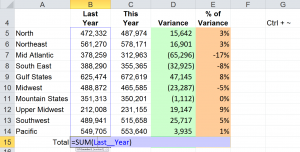
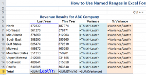
In my opinion, there are three reasons to use Named Range references in Excel Formulas:

  1. They are easier to write. Particularly, if you are referencing cells in another worksheet.
  2. They are easier to remember. Using =Sales – Cost of Goods Sold to determine Gross Profit vs. =A1 – B1
  3. They are easier to explain. Especially, if you are sending an Excel Workbook to a client or a colleague.

Creating Named Ranges in Excel

In this tutorial, I demonstrate two methods for creating a named range:

  1. Select the cells in the range and then type the name in the “Name Box” in the Upper Left Corner of the worksheet.
  2. Select both the cell with the “Name” and the adjacent cells for the range. Then use the Keyboard Shortcut Ctrl + Shit + F3 to open the Create Names from Selection Dialog Box

Remember that all Named Ranges MUST begin with a Letter or an Underscore and they CANNOT contain any Spaces!

Paste Named Ranges into Formulas

If you are using Excel 2007 or Excel 2010, you can take advantage of Formula AutoComplete to quickly and accurately include named ranges in your formulas. In ALL versions of Excel you can use the F3 Keyboard Shortcut to open the Paste Names Dialog Box and select the named range that you wish to paste into your formula.

Additional Resources for Excel

I invite you to visit my secure online shopping website – http://shop.thecompanyrocks.com – where you can preview all of the resources that I offer you.

Watch Tutorial in High Definition

Follow this link to watch my Excel Video in High Definition. My YouTube Channel – DannyRocksExcels – has received over 1 million views!

Watch Video Now

Share and Enjoy:
  • Add to favorites
  • Facebook
  • Twitter
  • Technorati
  • Print
  • email
  • Digg
  • StumbleUpon
  • del.icio.us
  • Yahoo! Buzz
  • Google Bookmarks
  • Orkut
  • SphereIt
  • Sphinn