DannyRocksExcels on YouTube Recognized as a Top 10 Channel for MS Excel Tutorials

Top 10 Sites for Excel Tutorials

Top 10 Sites for Excel Tutorials

I was thrilled to see this list – posted on Facebook – that recognized my YouTube Channel, DannyRocksExcels, as one of the Top 10 Sites for Microsoft Excel tutorials!

See the Complete List – Top 10 YouTube Channels

Click here to see the list of the Top 10 YouTube Channels for Excel Tutorials. I am honored to be included in this list!

Visit My YouTube Channel – DannyRocksExcels

I invite you to visit my DannyRocksExcels Channel on YouTube.

DannyRocksExcels

DannyRocksExcels on YouTube

As of today, I have published 250 Video Tutorials on YouTube. Many of my videos can be viewed in High Definition.

My videos have been viewed nearly 1.9 million times and my list of subscribers is close to 4,000.

My Top 10 Videos – The Last 7 Days

Here is a list of the 10 Most Viewed Excel Tutorials at DannyRocksExcels over the last 7 days – dating back from August 17, 2012. I have created Hyperlinks for each video. Just click on the title that you want to watch on YouTube:

  1. How to Use Advanced Filters in Excel
  2. How to Merge Multiple Excel Workbooks to a Master Budget
  3. Compare Two Excel Lists to Spot the Differences
  4. Use the Built-in Data Form in Excel to View and Filter All Fields for a Record
  5. How to Add a Check Box Control to an Excel Form
  6. How to Create a Summary Report from an Excel Table
  7. How to Create an Interactive Excel Pivot Chart
  8. Create Interactive Excel Forms by Including Option Buttons
  9. How to Use an Excel Data Table for “What-if” Analysis
  10. How to Calculate Overtime Hours on a Time Card in Excel

Shop at My Secure Online Website

I invite you to visit my secure online shopping website – http://shop.thecompanyrocks.com – to preview all of the Training Resources that I offer you.

How to Combine 2 Excel Workbooks Using VLOOKUP Function

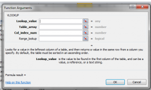
VLOOKUP Function Arguments

VLOOKUP Function Arguments

I created this video tutorial to assist one of my viewers. He had 2 Excel Workbooks that he needed to combine. Because he had a MemberID Field in each workbook, I decided that the VLOOKUP() Function would be the fastest way to complete this task for my viewer.

Tips Covered in this Video

  • Move or Copy a Worksheet to another Excel Workbook
  • Use a Mixed Cell Reference – e.g. $A4 – so that column “A” reference is “frozen” when copying formula
  • Create “Named Range” to use as the “Table_Array” argument in VLOOKUP
  • Use FALSE as 4th (optional) argument in VLOOKUP to produce an “exact match”
  • Use IFERROR to prevent “error messages” from displaying

Watch this Video in High Definition

Click on this link to watch this Excel Tutorial  in High Definition on my YouTube Channel – DannyRocksExcels

Learn About My Training Resources

I invite you to visit my secure online shopping website – http://shop.thecompanyrocks.com – to learn about the many training resources that I offer for sale.

Watch Tutorial Now


How to Use Excel’s Histogram Tool and The 80/20 Rule of Analysis

Histogram Charts in Excel

Excel Histogram Charts

This is the Third – and final – episode in my “Creating Frequency Distribution Reports in Excel” series of tutorials.  In this episode, I demonstrate a very powerful – and very easy to use – analysis tool – The Histogram Tool.

Excel’s Analysis ToolPak “Add-in”

This tool is included in the Analysis ToolPak which is an “Add-in” program within Excel. Beginning with Excel 2007, the Analysis ToolPak is automatically included in a basic installation of Excel. However, if you are using an earlier version of Excel or if, somehow, this Add-in has been disabled, I show you how to “activate it.”

Advantages of Using Excel’s Histogram Tool

  • No Formulas to write
  • Results are Numeric Values – not Formulas
  • Chart(s) can be added automatically
  • Multiple Chart Options
  • Pareto Chart Option

What is a Pareto Chart?

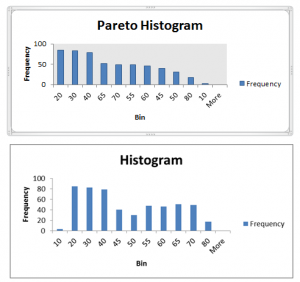
Pareto Analysis is commonly known as “The 80 / 20 Rule.” A brief explanation is: Roughly 80% of your sales come from only 20% of your customers or 20% of your products. I like to say, “You can focus on the Vital Few and not on the Trivial Many,” when you use Pareto Charts. As you will see in my video, when you choose the Pareto Chart option, the Histogram automatically sorts the Frequency Field in descending order and charts this field.

Links to All Videos in Frequency Report Series

Improve your Excel Skills – My Video Tutorials

I invite you to visit my secure online shopping website to see the many training resources that I offer. For example, click here to learn about my best-selling DVD-ROM, “The 50 Best Tips for Excel 2007.”

Follow The Company Rocks on Facebook

You can now follow me on Facebook – www.facebook.com/TheCompanyRocks


My Top 10 Most Viewed Excel Tutorials on YouTube Year-to-Date in 2012

DannyRocksExcels on YouTube

DannyRocksExcels on YouTube

Later this month, my YouTube Channel – DannyRocksExcels – will surpass 1.8 million views! Thanks to everyone who has visited, watched, and commented on my Excel video tutorials these past four years!

Top 10 Most Viewed Videos – January thru July, 2012

According to my YouTube statistics, these are the 10 most viewed Excel video tutorials on my channel. Click on the Links to watch any video on YouTube :

  1. How to Merge Multiple Excel Workbooks to a Master Budget – views year-to-date 39,338
  2. How to Use Advanced Filters in Excel – views year-to-date 29,700
  3. How to Use an Excel Data Table for “What-if” Analysis – views year-to-date 27,301
  4. How to Add a Check Box Control to an Excel Form – views year-to-date 27,171
  5. Consolidating Data from Multiple Excel Worksheets by Position – views year-to-date 26,517
  6. How to Create an Interactive Pivot Chart – views year-to-date 24,858
  7. Compare Two Excel Lists to Spot the Differences – views year-to-date 23,826
  8. Create Interactive Excel Forms by Including Option Boxes – views year-to-date 20,665
  9. How to Use the VLOOKUP Function in Excel – views year-to-date 20,574
  10. Import Excel Data Into MS Access – views year-to-date 18,288

Learn More Tips, Tricks, and Techniques for MS Office Programs

The 50 Best Tips DVD-ROMs

The 50 Best Tips Series of DVD-ROM’s

I invite you to visit my secure online shopping website – http://shop.thecompanyrocks.com – where you can purchase my video training resources.

The 50 Best Tips, Tricks & Techniques Series

Click on the link to go directly to the information page for each title. You will see a list of the 50 Tips and Ru Times for each title:

100% Satisfaction Guaranteed!

I stand 100% behind the quality of my products. I will refund your purchase price if, for any reason, you are not 100% satisfied – with no questions asked!

Thank you for your support through the years!

Danny Rocks

The Company Rocks

How to Use an Array Function in Excel – Learn How to Use the Frequency Function

Key Points for Frequency FunctionIn my experience, most of the people who I train have never heard of – let alone use – Array Formulas and Functions in Excel. However, once I demonstrate how they work, they become “hooked” and want to learn more about these “Magic Formulas!” In this tutorial, I demonstrate, “step-by-step” how to use the FREQUENCY() Function in Excel.

Previous Tutorial on The Company Rocks Website

If you watched my previous tutorial, I used the same data set and a Pivot Table to Group these 500 plus Sample Records by Age Bracket. Using a Pivot Table, you can quickly “group”  ages into brackets – without writing a single formula! However, on the down side, you must use a consistent “step-value” for these groupings – in this case by 10 years. When you need more flexibility in organizing your Age Brackets, use the Frequency Function in Excel.

How to Use the FREQUENCY() Function in Excel

  1. Create your “Bin Array.” In this example, enter – in ascending order – the ages that you want to find the “frequency of occurrences” between
  2. Select the “Array of Cells” that will contain your FREQUENCY() Function results.
  3. Write the FREQUENCY() Function –  1st argument is the  “Data_array”. In this case, I created a Named Cell Range called “Age.” this is mu “Best Practice Tip!”
  4. The 2nd argument is the “Bin_array.” Choose the vertical range of cells that you created in step 1 of this list. Make sure that the “size” of this Array matches the “size” of your Array Formula Selection.
  5. Complete the Array Function with the keyboard combination of “Ctrl + Shift + Enter.” This “CSE” combination is essential when entering all Array Formulas and Functions!

My Secure Shopping Website

I invite you to visit my secure shopping website – http://shop.thecompanyrocks.com – where you can preview all of the training resources that I offer. If you want to learn more about formulas and function, I offer a great resource: “The 50 Best Tips for Excel 2007.” Regardless of the version of Excel that you are currently using, you will pick up many great tips to improve your Excel skills!

Watch Tutorial in High Definition

Follow this link to watch this Excel Tutorial in High Definition on my YouTube Channel – DannyRocksExcels.

View My Tutorial Now on YouTube


How to Group People by Age Bracket Using an Excel Pivot Table

Pivot Table for Age Brackets

Pivot Table to Group Age Brackets

In my previous Excel Tutorial, I demonstrated how to use the Group Field command in a Pivot Table to summarize time periods by the Hour. Several viewers wanted to know what other grouping possibilities are available in Pivot Tables. One viewer wanted to know how to group people who responded to a survey by Age Brackets. That is why I created this tutorial!

Use DATEDIF Function to Calculate Age

From my perspective, the DATEDIF() is an invaluable function. However, it is not documented in Excel. Watch how I use its three arguments to calculate the age of each person in the data set.

Group Field by Age

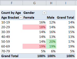
Select a single value in the “Age” Field and then select the “Group Field” Command. In the dialog box, choose the “step-value” for your groups. In this case, I chose the Default Setting of 10 years.

Show Pivot Table Values As

Some of the most powerful Pivot Table tools are found on the “Show Values As” tab of the “Value Field Settings” Dialog Box. Watch me demonstrate how to show each Age Bracket as a Percentage of the Column.

Apply Conditional Formatting to Pivot Table

Take advantage of the greatly improved Conditional Formatting Commands in Excel 2007 and Excel 2010 to focus attention on the key information in your Pivot Table. In this case, I use the “Top 10 Items” rule to apply Conditional Formatting to the two highest Age Brackets- by percentage – for each gender.

Learn Excel Pivot Tables Quickly

Follow this link to learn about the focused 90 minute video tutorials that I have published to help you to really learn how to get the most out of Pivot Tables. Available in versions for Excel 2003, Excel 2007, and Excel 2010.

Watch Tutorial in High Definition

Click on this link to watch this Excel Tutorial in High Definition on my YouTube Channel – DannyRocksExcels


How to Group an Excel Pivot Table Field to Summarize By Hours

Pivot Table Summary Report By Hour

Pivot Table Summary Report By Hour

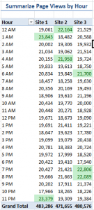
After viewing my previous video tutorial, one of my subscribers asked me to demonstrate how to actually summarize a minute-by-minute Excel report into an hour-by-hour report.

My viewer was unfamiliar with Pivot Tables – as are many Excel users – so I created this video to show him – and you how to do this.

Group a Pivot Table Field

Begin by right-clicking a single cell in the Time Field and choosing Group Field. In the dialog box, deselect Month and choose Hour. That’s it – it’s that simple!

Apply Conditional Formatting to the Top 10%

Beginning with Excel 2007, Conditional Formatting has been tremendously improved. Watch how I apply a “Top 10%” Conditional Format Rule with three mouse clicks!

Purchase My 90 Minute Focused Pivot Table Tutorial

Whether you are a novice or an experienced user of Excel Pivot Tables, you will learn some great Tips and Techniques when you purchase my 90 minute video tutorial: “Summarize, Analyze and Present Information with Excel Pivot Tables.”

Follow this link to learn more about my video tutorial for Pivot Tables. Available for ALL versions of Excel as either a DVD-ROM or as a Downloadable Product.

Watch Video Tutorial in High Definition

Click on this link to watch this Excel Video Tutorial in High Definition on my YouTube Channel – DannyRocksExcels


How to Create a Series of 30 Minute Time Intervals in Excel

How Excel Stores TimeOne of my readers tracks data points at 30 minute (half-hour) periods throughout the day. He asked me for some help in streamlining this process.

AutoFill the Step-value for a Series

You can use AutoFill in Excel to create this series. Here are the steps to take:

  1. In two adjacent cells, enter the beginning time value and the time that is 30 minutes later than the beginning time value.
  2. Select BOTH cells and AutoFill the cells in the range that you want to “populate.”

Calculate Decimal Number that Represents 30 Minutes

You can calculate the numeric value for a half-hour (30 minute) period:

  1. Use a Formula to subtract the Start Time from the End Time.
  2. Format the result as a Number with 6 Decimal Places.

In this case, the result is: 0.020833 which you can use as a Constant Value in a Formula.

Keyboard Shortcut to Enter the Current Time

Ctrl + Shift + : (Colon) will “time stamp” a cell.

How Excel Stores Time

While you can Format Time in a variety of ways, Excel must be able to recognize and store Time entries as Numeric entries! This means that correctly entered times align to the right-side of the cell. Time values are stored as a “decimal part of one” day. For example, 12:00 PM (Noon) is stored as 0.50 – 50% of the day has elapsed

Shop at My Secure Online Website

I invite you to visit my secure online shopping website – http://shop.thecompanyrocks.com – to view all of the resources that I offer you to improve your Excel skills.

Watch Tutorial in High Definition

Click on this link to watch this Excel Tutorial in High Definition on my YouTube Channel – DannyRocksExcels

How to Calculate the Calendar Year Quarter for a Date in Excel

Formulas to Calculate a Calendar Year Quarter

Formulas to Calculate a Calendar Year Quarter

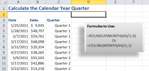
After watching my previous video tutorial, “How to Place Dates in a Fiscal Year Quarter,” several viewers requested that I demonstrate how to calculate the calendar year quarter for a date.

This requires “nesting” the MONTH() /3 Function inside either the ROUNDUP() or the CEILING() Function. I break these formulas down step-by-step in this video so that you can see how they work.

Formatting Numbers to Include Text

As a bonus, I demonstrate how to format the formula result cells to include the text “Quarter.” This is really simple to create as a custom format.

Download this Video Podcast from iTunes

You can watch and download this – and many of my – video tutorials for free at iTunes. Here is the link to my iTunes video podcast, “Danny Rocks Tips and Timesavers.”

Watch Video in High Definition

Follow this link to watch this Excel Tutorial in High Definition on my YouTube Channel – DannyRocksExcels

Visit my Secure Online Shopping Website

I invite you to visit my online shopping site – http://shop.thecompanyrocks.com – to preview and purchase my training resources. I guarantee your satisfaction 100%. I will refund your purchase if, for any reason, you are not satisfied with my products!


How to Place Dates in a Fiscal Year Quarter

Many organizations operate in a Fiscal Year – for example, April 1 through March 31 of the next calendar year. I get many requests from viewers for help with placing calendar dates into the proper Quarter for their Fiscal Year.

Excel Functions Used in Video TutorialWhile researching a question from one viewer, I cam across a very interesting formula that nests the “undocumented” DATEDIF() Function inside the CEILING() Function. I found this formula in the book, “Formulas and Functions with MS Excel 2003,” written by Paul McFedries. It is a very efficient formula.

What is Covered on the Video

Watch this video tutorial as I break down each step. As a Best Practice, I recommend that you break down a complex formula by working from the “inside out.” I start with the “nested” DATEDIF() function and then demonstrate the results of each formula detail.

Learn More About the “Undocumented” DATEDIF() Function

For various reasons, Microsoft does not offer any help or documentation for the very useful DATEDIF() Function. In fact, it is not even listed as a Function! However, it is very useful and often found in VBA (Visual Basic for Applications) coding. Here, are links to two videos that I created to help you understand how to use DATEDIF():

Learn How to Calculate a Calendar Year Quarter

In response to viewer requests, I created a companion video tutorial -” How to Calculate a Calendar Year Quarter in Excel.”

Resources Available at The Company Rocks

I invite you to visit my secure online shopping website – http://shop.thecompanyrocks.com – to preview the many resources that I offer for helping you to improve your software skills.

Watch Video Tutorial in High Definition

If you would like to watch my video tutorial for “Finding the Fiscal Year Quarter for any Date,” click on this link. I have posted it on my YouTube Channel – DannyRocksExcels

Watch this Video Now