Archives for 2011

20 Tips for Delivering a Successful Presentation

Presenting to Group

Presenting to Group

Have you been asked to speak or deliver a presentation at an upcoming event? Once you have accepted the invitation to speak or present, you need to start preparing. Where do you begin?

Successful presenters follow a process. They have a system which they have developed over the years. They use a checklist of Best Practices to help ensure that they deliver successful presentations every time!

So, you may be asking … “Where do I get a list of tips? Has someone created a checklist that I can use?”

Fortunately, you have come to the right location! I have created a checklist of “20 Tips for a Successful Presentation” that you can download – for free!

Click on this link to download my 20 Tips for a Successful Presentation as an Adobe PDF.

Here is my list of the 20 Tips that I use whenever I speak or deliver a presentation. These are also the tips that I share with my clients when I coach them to deliver successful presentations.  You will learn about:

  • How to discover your “Words-per-Minute” (WPM) Count
  • The “B-L-O-T” (Bottom Line On Top) Technique
  • The “Power of the Pause”

And 17 additional tips. Be sure to download the complete checklist  of  “20 Tips for a Successful Presentation” to get more information about each tip:

Tips While Preparing Your Presentation

  • Tip #1 – Prepare with your audience in mind
  • Tip #2 – Begin your presentation with “The End in Mind”
  • Tip #3 – Use the classic model to structure your presentation
  • Tip #4 – Prepare by writing out your presentation

Click on this link to download your copy of my 20 Tips for a Successful Presentation

Tips for Delivering Your Presentation

  • Tip #5 – Memorize two sections of your presentation
  • Tip #6 – Communicate and confirm your equipment needs in advance
  • Tip #7 – Get comfortable with the physical setting
  • Tip #8 – Your audience will “Tune-in / Tune out” during your presentation
  • Tip #9 – Remember the “Power of the Pause!”
  • Tip #10 – Maintain Eye-contact with your audience
  • Tip #11 – Pace your presentation

Follow this link to download a PDF of my 20 Tips for a Successful Presentation

Tips for PowerPoint

PowerPoint Tips

Tips for Creating PowerPoint Slides

  • Tip #12 – You are the Presentation!
  • Tip #13 – Do not write complete sentences on your slides!
  • Tip #14 – Take advantage of the “White Space” on your slides
  • Tip #15 – Choose appropriate visual images

Want to get a copy of this checklist – complete with details for each of these tips? Click here to download 20 Tips for a Successful Presentation as a PDF.

Do you want to learn how to use PowerPoint effectively? Click on this link to learn more about my DVD-ROM, “The 50 Best Tips for PowerPoint 2007”

Tips for Engaging Your Audience

  • Tip #16 – Phrases to avoid
  • Tip #17 – Phrases to substitute
  • Tip #18 Encourage audience questions
  • Tip #19 – Audiences remember stories

Get your free copy of this checklist. Click on this link to download 20 Tips for a Successful Presentation

Tip for Delivering a Successful Presentation

  • Tip #20 – Visualize your Successful Presentation!

So, there is the checklist that I use. Be sure to download your copy to learn more about each of these “20 Tips for a Successful Presentation.”

Do you have a favorite tip? What works for you? Add your comment in the area below this article. Or you can send it to me via email: danny@thecompanyrocks.com

Read or Forward this Article from Ezine Articles Website

A variation of this article is purclished on the Ezine Articles Website  – www.ezinearticles.com where you can read it or forward it to your friends and colleagues. Click here for the direct link to the article.

Invitation to Visit My New Online Shopping Website

I have just opened my new, secure online shopping website. I invite you to visit http://shop.thecompanyrocks.com to see all of the products and resources that I offer.




Tips for Working with Array Formulas and Functions in Excel

Using ARRAY Functions in Excel

ARRAY Formulas in Excel

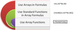
Array Formulas and Functions are very powerful tools to use in Excel. However, the concept of working with ARRAYs take a little bit of time and practice. In this video tutorial, I demonstrate how to:

  1. Create formulas that use ARRAYS as arguments
  2. Work with ARRAY FUNCTIONS – for example, the TRANSPOSE Function
  3. Key “Got’cha” steps to master – for example, selecting all cells to receive formula results before creating the ARRAY Formula.
  4. The importance of using Ctrl+Shift+Enter to complete the Array formula.

What is an ARRAY?

“An Array is a collection of Cells or Values that Excel treats as a single unit.”

Why Use an ARRAY Formula?

  1. Automatic Level of Protection for Formula Cells – You cannot delete nor edit a single cell in an Array Formula
  2. Eliminate Intermediary Calculations – For example, you can find the Grand Total without having to create a field to calculate “Extended Price.”
  3. Worksheet, usually, calculates faster because you are using fewer formulas.

Visit My NEW Online Shopping Website

http://shop.thecompanyrocks.com is my new, secure online shopping website. I invite you to visit and preview my new products.

Watch Tutorial in High Definition

Follow this link to view this tutorial in High Definition on my YouTube Channel – DannyRocksExcels

How to Use the Offset Function Inside a VLookup in Excel

Vlookup in Excel

VLOOKUP in Excel

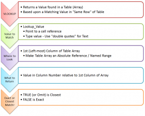
Each month, I get 5 to 6 emails of phone calls from viewers who who are having trouble using the VLOOKUP Function in Excel. In the majority of cases, the problem is that their Data Table is setup so that the “Key” field that they need to search in is NOT the Left-most or first field in the table. It is not always practical – nor desirable – to use “Cut and Paste” to rearrange the fields in the data set. So, what techniques can you use to fix this?

Use the OFFSET Function Inside a VLOOKUP Function

In this scenario, our IT Department sends us a daily report of the products that we sell including fields for the current cost and quantity on-hand. We use this report to generate additional reports and filters. This report gets saved automatically as an Excel 2010 Table with the name “Inventory.” The problem is, whenusing a VLOOKUP, that the first – or Left-most – field is NOT the “Key” field that we want VLOOKUP to use to search for a Match in order to return the current price or inventory for individual product.

The OFFSET() Function in Excel, makes it easy to reference a “starting field” that, in this case, is one column to the Right. This is perfect for our situation. We can continue to use our “named range” with the VLOOKUP!

Watch Video in High Definition

Follow this link to watch this tutorial in High Definition on my YouTube Channel – DannyRocksExcels

Visit My New Secure Online Shopping Website

I invite you to visit my new online shopping website at: http://shop.thecompanyrocks.com I have created new, extended length video tutorials that you can either purchase to download immediately or order them on a DVD-ROM. In addition, I have published versions of my 90 minute Pivot Tables Video Tutorials for Excel 2003, Excel 2007 and Excel 2010. So, I have the tutorials that you want for the Excel version that you are currently using!

Click to Play Excel Video Tutorial

Structured Formula References in Excel 2007 and Excel 2010 – Part 2

Compare Structered References Excel 2007 v 2010

Compare Structured References 2007 v 2010

This is the second and concluding part of this series where I demonstrate how to use Structured Formula References when referring to Excel Tables.

Key Points Covered

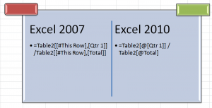
  • The difference between Structured Formula References in Excel 2007 and Excel 2010
  • How to Edit Structured Formula References
  • How to Write Structured Formulas using the new Formula AutoComplete drop-down menu


Watch My Video Tutorial Now


Watch Video in High Definition on YouTube

Click on this link to watch this Video in High Definition on my YouTube Channel – DannyRocksExcels

Go to Part 1 in this Series of Video Tutorials

Follow this link to go to Part 1 in this Series of Tutorials about using Structured Formula References in Excel Tables.

Visit My New Secure Online Store

I have just published 6 New Products and opened a new, revised, secure online shopping website. Take a look at: http://shop.thecompanyrocks.com


Master Excel Pivot Tables in 90 Minutes: Announcing My New Extended Length Video Tutorials!

Master Pivot Tables in Minutes

Master Pivot Tables in Minutes

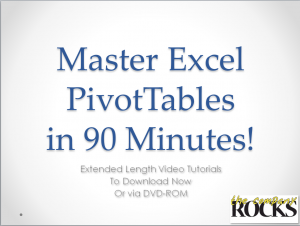
I am proud to announce the publication of my new series of “Extended Length” video tutorials: “Master Excel Pivot Tables in 90 Minutes!”

Now, you can can get an in-depth video tutorial, so that you can Master Excel Pivot Tables with 90 minutes of video instruction. You also receive the actual Excel Workbook file that I used while filming the video lessons as well as a printed step-by-step instructional manual.

What Makes this Product Unique?

  •  Excel Versions for the Video Tutorials

  • Available for Excel 2010, Excel 2007 or Excel 2003

Multiple Options for Delivery

Resources to Assist Your Learning

  • The Excel Workbook file that I used while filming each video lesson – Included with purchase!
  • PDF Manual of Step-by-Step Instructions – That you can print out – Included with purchase!

Take a Short Video Tour

Follow this link to watch a short – 5 minutes – video tour of my new products on my YouTube Channel – DannyRocksExcels

Visit My New Secure Online Shopping Website

I invite you to visit http://shop.thecompanyrocks.com This is my new online shopping website. I have created secure shopping carts to ensure that your privacy is protected. I also offer a 100% Customer Satisfaction Policy. If, for any reason, you are not 100% satisfied with any of my products, I will refund your purchase with no questions asked!

Danny Rocks

The Company Rocks

How to Use Structured Formula References for Tables in Excel 2007 and Excel 2010

Structured Formula Reference - Excel 2007

Structured Formula Reference - Excel 2007

Beginning with Excel 2007, you can – and should – convert a Standard Data Range to an Excel Table. Doing so offers several advantages:

  • You get a selection of Table Styles – including Alternate Row Shading – that make it easier to read your tables.
  • You can automatically extend the Scope of your Table – by adding additional Fields (Columns) or Records (Rows).
  • You can give your Table a “Name” to reflect the purpose of the Table.
  • You can add a Total Row to Subtotal each Field (Column) and you can change the Function used to Subtotal from a drop-down menu.
  • You can apply Structured Formula References in the Table – Enter the Formula in a Single Cell and it is Automatically copied down for each record in the Table.

“In This Row” Formula Styles

Structured Formula References use a new style of formulas. Rather than referring to a specific Cell, in an Excel Table, you refer to a Field “in this row.” This type of formula is easy to create “inside the table.” It is also fairly easy to create “outside the Table” using the new Formula AutoComplete tool. You will be using [ ] (Left & Right Brackets) for these formulas. I go over these details, in-depth, in this video tutorial.

There are also distinct differences in how Structured Formula References are created between Excel 2007 and Excel 2010. These Structured Formula References are greatly streamlined in Excel 2010 – in my opinion.

The SUBTOTAL() Function and Excel Tables

I strongly recommend that you become familiar with how to use the valuable SUBTOTAL() Function in Excel when referring to the data in a Table. With the SUBTOTAL Function, you can produce a wide range of summaries anywhere on your Excel Workbook. And… the Subtotal Results reflect the totals for any “Filters” that you apply to your Table.

Play this Video in High Definition

Watch this Video in High Definition

Follow this link to watch this Excel Tutorial in High Definition on my YouTube Channel – DannyRocksExcels

Go to Part 2 in this Series of Tutorials

Follow this link to go to Part 2 in this series of tutorials about using Structured Formula References in Excel Tables.

Announcing 6 New Products on My New Online Secure Shopping Website

I invite you to visit my new online shopping site. I have added 6 new products – Extended Length Video tutorials that you can either “download now” or purchase as a DVD-ROM. Each product contains over 90 minutes of in-depth video instruction for Pivot Tables. You can choose the product to fit your version of Excel – Separate products for Excel 2003, Excel 2007 and Excel 2010.

Click here to view my new products.

How to Use the Show As Values Dialog Box for an Excel Pivot Table

Show Values As for Pivot Table

Show Values As for Pivot Table

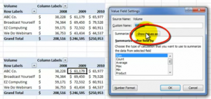
I created this Excel Video Tutorial in response to a viewer who wrote to me about a problem that he was having with an Excel 2007 Pivot Table.

Viewer’s Question

“I want to show both the % of Growth from Fiscal Year-to-Year and the Actual Variance in Volume between each of 3 Fiscal Years. I have been trying to do this with a Pivot Table Calculated Field, but I am not having any luck with this approach. What do you suggest?”

My Solution

Use the “Show values As” Dialog Box which you find in the Value Field Settings Dialog Box. I continue to be amazed, when I teach Pivot Tables in a Live Seminar, that the high majority of my students have never clicked on this Tab!

In this case, we are working with a “copy” of the original Pivot Table. Simply choose “% Difference From” in the drop-down menu. Next, choose Fiscal Year and Previous (year) to create a Fiscal Year-over_Fiscal Year Report. It is so easy to do! And… you do not have to write a single formula to create this report!

Watch Video Here on My Website


Watch Excel Tutorial in High Definition

Follow this link to view this Excel Tutorial in High Definition Mode on my YouTube Channel – DannyRocksExcels

Master Excel Pivot Tables in 90 Minutes!

Follow this link to learn about my new extended length (90 minutes) Pivot Table Video Tutorials

How to Take Advantage of the Go To Special Dialog Box Options in Excel

Go To Special Options

Go To Special Options

In my opinion, the Go To Special Options Dialog Box offers some of the most useful tools in Excel!

Why?

Because,  you must…

Select Cells Before Performing an Action on these Cells

The “key” to understanding ANY MS Office or Windows Program is… You MUST select a single cell or a range of cells BEFORE you can perform an action on them – e.g. Formatting you selection, deleting your selection, editing your selection or auditing your selection.

Tips Presented in this Video Tutorial

  • Select cells with Comments – so that you can “format” these cells to make them easier to identify.
  • Select cells that contain Constant Numeric Values – so that you can easily “spot” cells that should – bu do not – contain formulas.
  • Select cells that contain Specific Types of Formulas – e.g. Text Formulas – to “audit” your formulas.
  • Find the “Last Cell” in your worksheet – the last cell that contains EITHER content OR FORMATTING – This can be an “eye-opener!” for you.
  • Select the cells that contain Data Validation – perhaps you failed to “validate” all of the cells in a range.
  • Select the cells that contain Conditional Formatting – perhaps your did not select ALL of the cells in a Range BEFORE you applied a Conditional Formatting RULE!
  • Learn how to select the “Visible Cells Only” before performing a copy and paste operation – especially helpful when copying the “collapsed cells” for an Excel Outline.

I am positive that Excel users at ANY LEVEL will be able to pick up at least one solid tip from this Video Tutorial. Please send me your comments to let me know what you learned – or what you need clarification on.

Watch Tutorial in High Definition Mode

Follow this link to view this Excel Tutorial in High Definition / Full Screen Mode on my YouTube Channel – DannyRocksExcels

Learn About My New Extended Length Excel Video Tutorials

I have just published the first in a series of “Extended Length” – 90 Minutes – Video Tutorials, “Excel Pivot Tables to Summarize, Analyze and Present Your Data.” Follow this link to learn more about this tutorial. I have created separate versions of the tutorial for Excel 2010, 2007 and 2003.

How to Use the Solver Add-in for Excel – Part 2

Solver Parameters

Solver Parameters

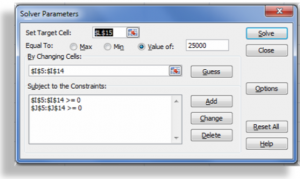
This is Part 2 of my series of video tutorials where I demonstrate how to use the SOLVER Add-in Tool in Excel to produce a specific result for a formula.  Remember that SOLVER is an Add-in program that you must activate before you can use it. Watch Part 1 in this series to learn how to activate SOLVER.

In this tutorial, I work with the same data set that I used in Part 1. This time, I want to achieve a specific amount of Gross Profit Sales Dollars. First, however, I must determine what is a reasonable amount to set as the Target for Solver to return.

Use SUMPRODUCT Function in Excel

I use the SUMPRODUCT Function to quickly determine my possible Revenue, Cost of Goods Sold and Gross Profit is I sell all of the Units that I have in stock. Now, I have a reasonable Target for SOLVER to reach. SUMPRODUCT is a very efficient Function that, unfortunately, very feel Excel users – in my experience – know about. Follow this link to my Index of Excel Video Lessons to find additional tutorials for SUMPRODUCT.

Best Practice Tips for Solver

  • Work with a copy of your worksheet. This is always a good idea, and it is most important when you are beginning to learn how to work with SOLVER.
  • Write out your Goal for SOLVER.
  • Do you want SOLVER to Maximize the Formula? For example, to Maximize your potential profit?
  • Do you want SOLVER to Minimize the Formula? For example, to Minimize your costs?
  • Do you want SOLVER to return a Specific Number? If so, what is that number?
  • Determine your “Variable Cells.” SOLVER calls them the “By Changing Cells.” These are the cells that SOLVER will automatically adjust.
  • The Variable Cells must “feed int” the formula in your Target Cell – This is the key to making SOLVER work!
  • Write out your “Constraints.” These are the “real-world” conditions that you want SOLVER to operate under. This is the real power in SOLVER.
  • Do not treat the SOLVER results as “the Gospel.” SOLVER is a powerful Business Intelligence Tool. You, however, know your own business or industry. Use SOLVER as a tool to help you to make informed business decisions.


Watch Part 1 in SOLVER Series of Video Tutorials

Watch Tutorial in High Definition

Follow this link to view this Excel Tutorial in High Definition on my YouTube Channel – DannyRocksExcels.

How to Use the SOLVER Tool in Excel to Produce the Optimal Result for a Formula

Key Points for SOLVER

SOLVER in Excel – Key Points

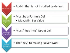
I am responding to a “flurry” of requests to produce an Excel Video Tutorial that demonstrates how to use the SOLVER TOOL in Excel. Here are the key points to remember when you want to use the SOLVER Tool:

Activate the SOLVER Tool

SOLVER is an “Add-in” tool that needs to be “activated” before you can use it. In Excel 2007 / 2010, you do this via Excel Options – Addi-Ins – Excel Options. In Excel 2003, you do this via the Tools Menu – Add-ins – Solver.

Prepare Data for Solver

In order to use the SOLVER Tool, you must:

  • Establish the “Target Cell.” This cell must contain a formula. This is the cell that you want to “optimize” by using SOLVER.
  • Determine the “By Changing” Cells. These are the cells that SOLVER will change in order to deliver the optimized result in the Target Cell. The “By Changing” cells MUST “Feed Into” the Target Cell.
  • Establish the CONSTRAINTS for SOLVER. This is the “key’ element that gives SOLVER its power. You can add as many constraints as needed. My recommendation is that you “write them out” before you start  to use the SOLVER Tool.

SOLVER is very powerful. However, you MUST “think it through” before you apply it. It will take lots of practice for you to understand how to properly set up your data to produce appropriate SOLVER results.

Part 2 in this Series of Tutorials for Solver in Excel

Here is the link to watch Part 2 in this Series of Tutorials about the SOLVER Add-in Tool in Excel

Download Excel Workbook for this Lesson

Follow this link to download the Excel Workbook that I used for this lesson. I store my uploaded Excel workbooks on my SkyDrive at www.office.live.com

View this Tutorial in High Definition

Click on this link to watch this Excel Tutorial in High definition / Full Screen Mode – on my YouTube Channel, DannyRocksExcels