Archives for 2011

How to Create a Summary Report from an Excel Table

Functions for Executive Summary

Functions for Executive Summary

I created this Excel Video Tutorial in response to a viewer who, in her company, is not permitted to use a Pivot Table to create a report. Unfortunately, this happens more often than you might think. Nevertheless, I promised to share my tips and advice. I think that many of this tips will help Excel users at all levels.

Tips Covered in this Video Tutorial

  • Use Advanced Filter to Extract a list of unique customer names from a range with @ 4,300 records.
  • Later in the lesson, I show you how to extract this list to a different worksheet – a tip that will save you time when preparing your reports!
  • How and why to convert a normal range of data into a TABLE in Excel 2007 / 2010 or into a LIST in Excel 2003.
  • How to create “Named Ranges” for your key data cells and to use them in your Formulas and Functions.
  • How to use the SUMIF, AVERAGEIF and COUNTIF Functions in your summary report.

Keyboard Shortcuts Used in this Tutorial

  • Ctrl + T to convert to a TABLE in Excel 2007 / Excel 2010
  • Ctrl + L to convert to a LIST in EXCEL 2003
  • Ctrl + A to open up the Function Arguments Dialog Box
  • Ctrl + Shift + F3 to open the Create Names Dialog Box
  • F3 to open the Paste Names Dialog Box

I decided that I will only make this video available on YouTube – I think that you will enjoy the clarity that you get from the High-Definition / Full Screen Mode.

Watch Tutorial in High Definition on YouTube

Follow this link to view this Excel Tutorial in High Definition on my YouTubeChannel – DannyRocksExcels

Visit my new secure online shopping website

I invite you to visit http://shop.thecompanyrocks.com – my new online shopping website.

Watch Video Now

How to Identify and Then Delete Duplicate Records in Excel

Identify & Delete Duplicates

Identify & Delete Duplicates

It is almost inevitable that, over time, your Excel data set will contain duplicate records. This can be costly – if the duplicate records are in your mailing list. And it can also result in errors when you count and calculate data.

Three Methods to Identify and Delete Duplicate Records

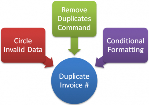
In this Excel Tutorial, I demonstrate three approaches to identify duplicate records in a data set:

  1. Circle Invalid Data – This tool works in coordination with Data Validation.
  2. Remove Duplicates – This powerful command was introduced in Excel 2007. It does not “preview” the records to be deleted, so my advice is to use this command with a copy of your data.
  3. Conditional Formatting – Greatly improved for Excel 2007 and Excel 2010. Now, you have a menu choice to apply conditional formatting to either Duplicate or Unique Records. If you are still using Excel 2003 or earlier, I show you how to write the formula needed to use Conditional Formatting to highlight duplicate records.

Watch The Tutorial in High Definition on YouTube

Follow this link to view this Excel Tutorial in High Definition on my YouTube Channel – DannyRocksExcels

How to Prevent Duplicate Entries in Excel with Data Validation

Formula for Data Validation

Formula for Data Validation

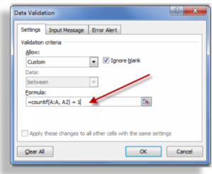
Over time, it is easy for duplicate entries to creep into an Excel Data Set. In this video tutorial, I show you, step-by-step, how to apply Data Validation to a range of cells so that anyone who attempts to enter a duplicate value will be prevented from doing so.

Use a “Logical Formula” for Data Validation

In this lesson, I show you how to “customize” the COUNTIF Function in the Data Validation Dialog Box so that it returns the value of TRUE. Logical formulas return either TRUE or FALSE. You MUST use a Logical Formula in Data Validation.

What Else is Covered in this Tutorial?

  • Use Paste Special – Validation to extend Data Validation to a wider range of cells
  • Use Find – Go to Special – Validation to highlight all cells on worksheet that contain Data Validation
  • Use Circle Invalid Entries from the Data Validation menu to automatically “draw a red circle” around existing cells that contain duplicate values
  • How to quickly remove Data Validation from a Range of Cells

Related Topic – Conditional Formatting in Excel

Another way to highlight existing cells that contain duplicate values is to use Conditional Formatting. The improvements in Excel 2007 and Excel 2010 make this “a snap” because this is now a Menu Selection! In my next tutorial, I will show you how this is done in both Excel 2003 – with the COUNTIF Function – and from the new Menu Selections introduced in Excel 2007.

Watch Tutorial in High Definition

Follow this link to my YouTube channel – DannyRocksExcels – where you can watch this tutorial in High Definition mode.

Keyboard Shortcuts to Enter and Edit Data Efficiently in Excel


Keyboard Shortcuts to Enter Data

Keyboard Shortcuts to Enter Data

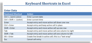
This is the latest installment in my series of video tutorials where I demonstrate how to use Keyboard Shortcuts in Excel. In this tutorial, I demonstrate how to Enter and Edit Data Efficiently in Excel using Keyboard Shortcuts.

Tips Covered on Video Tutorial

Here are the main Keyboard Shortcuts that I show you how to use on this video:

  • Enter Current Date in a cell.
  • Enter Current Time in a cell.
  • Use Ctrl + Enter to accept data entry and keep the focus on the current cell.
  • Use Ctrl + Enter to populate a range of selected cells.
  • Use Alt + Enter to “Wrap the Text” in a cell.
  • Use F2 to edit data inside a cell.
  • Use Ctrl + left & right directional arrows to move to the beginning of the next / previous word while editing in the cell.
  • Use ‘ (apostrophe) as the first character in a cell to make this a “text” entry.

Download my complete Chart of Popular Keyboard Shortcuts as a PDF 

 Follow this link to download – for free – my 5 Page Chart of Popular Excel Keyboard Shortcuts as a PDF.

Subscribe to my Video Podcast on iTunes

Here is the link to subscribe to my video podcast, “Danny Rocks Tips and Timesavers” on iTunes. It is offered for free!

Watch Tutorial in High Definition on YouTube

Follow this link to view this Excel Tutorial in High Definition mode on my YouTube Channel – DannyRocksExcels

How to Use Criteria in Excel Functions and Filters

Criteria for Advanced Filter

Criteria for Advanced Filter

When you apply a Filter to an Excel data set, you use Criteria. In a filter, only the records that can answer “TRUE” to the criteria that you set will appear. The records that answer “FALSE” are hidden while the filter remains in place.

Logical Functions

The IF(), AND() and OR() Functions belong to a group of Logical Functions. In their function arguments, they evaluate a “Logical Test” and can perform one action is the answer is “TRUE” and a different action if “FALSE.” 

  • The AND() Function – each of the Logical Tests must be met in order to return the answer “TRUE.”
  • The OR() Function – if any condition is met, the answer that is returned is “TRUE.”
  • I frequently “Nest” an AND() Function or an OR() Function inside an IF() Function to test multiple criteria.

Advanced Filters in Excel

While many Excel users are familiar with Filtering, in my experience, I find that many people get confused when it comes to using Advanced Filters. In this video tutorial, I try to eliminate this confusion. Watch and you will learn how to:

  • Write Criteria for Advanced Filters using “AND” criteria and “OR” Criteria.
  • Copy the “Filtered Records” to another location
  • Use the Keyboard Shortcut Ctrl + Shift + L to quickly “toggle” normal filter drop-down menus on or off.


Watch Tutorial in High Definition

Follow this link to watch this Excel Tutorial in High Defintion on my YouTube Channel – DannyRocksExcels

Record a Macro in Excel to Fix an Imported Text File

Macro Commands

Macro Commands

A viewer asked for my help in fixing a “Text” file that he imports into Excel each month. His IT department creates this file for him. The problem is that:

  • The Field Header Labels are arranged on two rows – He needs all of the labels to be on one row.
  • Each record is arranged on two rows – He needs each record to appear on one row.
  • There is a blank row separating each record  – He needs to remove all of the blank rows.

This is a perfect job for an Excel Macro!

In this tutorial, I first demonstrate how to create the Macro in Excel 2010. Then, I repeat the process using Excel 2003 – the version that my viewer is currently using.

Topics Covered in the Tutorial

  • Adding the Developer Tab to the Ribbon in Excel 2010
  • Creating back up copies of worksheets before recording the Macro
  • Using the Fill Across Worksheets (Grouped) to copy both content and formatting
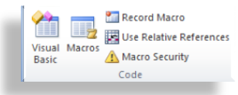
  • Using Relative References when Recording a Macro
  • Planning the steps you will take before Recording the Macro
  • Using Keyboard Shortcuts to Run the Macro
  • Creating and Editing a Command Button to Run the Macro
  • Viewing the VBA Code that Excel creates when you Record the Macro
  • Using Step Into to see how each step in the Macro is executed
  • Viewing and Changing Security Settings for Macros
  • Storing Macros in a Trusted Location (Excel 2007 and Excel 2010)
  • Saving Worksheets that contain Macros in Excel 2007 and Excel 2010

Watch Tutorial in High Definition

Follow this link to view this Excel Tutorial in High Definition mode on my YouTube Channel – DannyRocksExcels.

Excel Keyboard Shortcuts to Fill a Series

Here is the latest installment in my series of video tutorials on Keyboard Shortcuts in Excel. In this lesson, I demonstrate how to Fill a Series with Values or a Formula Down or to the Right.

The more interesting Keyboard Shortcuts that I demonstrate in this lesson are:

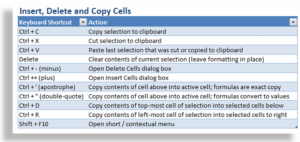
  • Ctrl + ‘ (apostrophe) – to copy the value from the cell directly above; to copy the formula from the cell directly above while retaining exact cell references.
  • Ctrl + Shift + ” (double quote) – to copy the value from the cell directly above; to copy the “result” of the formula from the cell directly above.

Download My Free “Chart of Popular Keyboard Shortcuts in Excel”

Watch Tutorial in High Definition

Click here to go to my YouTube Channel – DannyRocksExcels – where you can watch this tutorial in High Definition mode.


Excel Keyboard Shortcuts to Hide, Unhide, Insert and Delete Cells, Columns and Rows

Commands in Cells Group

Commands in Cells Group

Here is the latest installment in my series of video tutorials demonstrating how to use Keyboard Shortcuts in Excel. These Keyboard Shortcuts perform actions that you find in the Cells Group of commands on the Ribbon in either Excel 2007 or Excel 2010.

Topics Taught in Video Tutorial

Here are the topics that I teach in this tutorial. Using Keyboard Shortcuts to:

  • Select all cells in current row(s) Shift + Spacebar
  • Select all cells in current column(s) Ctrl + Spacebar
  • Open Insert Dialog Box Ctrl ++ (plus)
  • Open Delete Dialog Box Ctrl + – (minus)
  • Open short / contextual menu Shift + F10
  • Hide current row Ctrl + 9
  • Hide current column Ctrl + 0 (zero)

Download My “Chart of Popular Keyboard Shortcuts for Excel”

Click here to go to my Exclusive Membership Content page and download my charts of keyboard shortcuts. They are free to members who register.

Watch Video in High Definition

Follow this link to view this tutorial on my YouTube Channel – DannyRocksExcels

For some strange reason, I could not produce this video for my Podcast. So, the only way to view it is on YouTube.

Puchase My DVD-ROM

If you enjoy these tips. If you enjoy my style of instruction. Then, you will really benefit from purchasing and learning from my best-selling DVD-ROM, “The 50 Best Tips for Excel 2007.” 

Follow this link to learn more about my DVD-ROM and to open a Secure Shopping Cart to make your purchase.

How to Use Excel Keyboard Shortcuts to Cut, Copy and Paste Formulas and Formatting

Keyboard Shortcuts for Cut, Copy & Paste

Keyboard Shortcuts for Cut, Copy & Paste

In addition to showing you the Keyboard Shortcuts to Cut, Copy and Paste in Excel, I demonstrate how these actions affect formulas and formatting.

Topics in this Tutorial

Here are the topics that I demonstrate in this video tutorial:

  • Select multiple cells using the keyboard
  • Use Ctrl + Enter to update all cells in the selection
  • Use Ctrl + ~ to “toggle” between showing and hiding formulas in all cells
  • Use F2 to edit in the cell – and to diagram cell references for formulas
  • Use Ctrl + C to copy the “relative cell references” in a formula
  • Use Ctrl + X to cut an Excel formula that retains the original cell references
  • Open and use the Office Clipboard to store up to 24 most recent copy and cut items
  • Use Ctrl + Z to undo multiple actions
  • Use Ctrl + A to select all cells in a contiguous range
  • Use the Delete key to delete the contents of a cell or range while retaining the formatting
  • Use the Clear All command to remove both formatting and contents in a range of cells

Download My Complete Charts of Popular Keyboard Shortcuts

Follow this link to my Excelusive Membership Content Page where you can download all of my charts and tables of Keyboard Shortcuts.

Watch Video in High Definition

Follow this link to view this tutorial in High Definition on my YouTube Channel – DannyRocksExcels

How to Use Keyboard Shortcuts in Excel to Control Basic File Operations

Excel 2007 File Operations

Excel 2007 File Operations

If you have recently upgraded to either Excel 2007 or Excel 2010, you REALLY NEED to master the Keyboard Shortcuts that I present in this lesson!

Many Excel veterans who upgrade, tell me that they initially felt “lost” with the new user interface. Some of my clients called me in a panic because they didn’t know where to look to Print their work or to open a document. If you know how to use the Keyboard Shortcuts that I present in this lesson, you will never be at a loss. As an added bonus, these Keyboard Shortcuts work with ALL Microsoft Office programs and also for most Windows-based programs.

The “N-O-W-S” Keyboard Shortcuts

I use this acronym – NOWS – to remember the keyboard shortcuts to Open, Close and Save Documents in MS Office programs. Use Ctrl + W to Close the active worksheet.

In this video tutorial, I also show you when NOT to use Keyboard Shortcuts! There are many times when you need to access the full file menu selection.

Keyboard Shortcut for Print Preview

Use Ctrl + F2 to open up the Print Preview pane. Use the “Esc” key to Exit Print Preview.

Download My Chart of Popular Keyboard Shortcuts as a PDF

Follow this link to go to the web page where I store my Keyboard Shortcut Charts and other download-able content.

These Keyboard Shortcuts work for all versions of Excel. So far, I have found only one Keyboard Shortcut that is different when used in Excel 2007 / 2010 than in Excel 2003.

More Video Tutorials for Keyboard Shortcuts

This is the first in a series of video tutorials that I have planned. Each video will focus on the Keyboard Shortcuts you can use to perform a specific task – e.g. Formatting Cells, Inserting and Deleting, etc. My plan is to post one new video in this series per week.

Watch Video Tutorial in High Definition Mode

Follow this link to view this video tutorial in High Definition on my YouTube Channel – DannyRocksExcels