Excel VBA Macros | The Company Rocks

Danny February 12, 2013 Leave a Comment

How to Edit an Excel Macro that You Recorded

This is Part 3 in my series, “How to Record, Run, and Edit Macros in Excel.” In this episode, I demonstrate how to open up the VBA (Visual Basic for Applications) Code window and then:

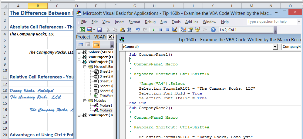
Step Into each line of the code – using the F8 Keyboard Shortcut – to examine how the Macro Behaves
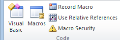
Use the ‘ (apostrophe) to “remark out” one line of the code. This will quickly change the macro to use Relative Cell Referencing rather than Absolute Cell Referencing!
Edit one line of the VBA Code to change the “text” that you want your macro to enter.

I created this series of Excel Tutorials to assist my viewers to “get started on the right path” when they first start to experiment with the power of Macros in Excel. I welcome your feedback on this – or any – Excel tutorial that I have published.

Step Into a Macro

When you run a Macro, it is impossible to “trouble shoot” or examine the individual actions that occur. In this lesson, I demonstrate how to use “Step Into” mode – with the keyboard Shortcut F8 – to run each line of the VBA Code step-by-step. Using Step Mode with any macro is a great way to learn how top efficiently write, record, or edit a macro.

Secure Online Shopping for Excel Training Resources

I welcome you to visit my Secure Online Shopping Site – http://shop.thecompanyrocks.com – where you can learn about the range of video training resources that I offer.

Watch Excel Tutorial in High Definition

Follow this link to watch my tutorial in High Definition on my YouTube Channel – DannyRocksExcels.

View Excel Video Tutorial Now

Share and Enjoy:

Filed Under: Excel Training, Excel VBA Macros Tagged: Excel Keyboard Shortcuts, Excel Video Training, Step into Macros, Turn on Relative Cell Referencing when Recording a Macro in Excel, VBA Code for Excel Macros, Video lessons for Excel, Visual Basic Editor

Danny February 6, 2013 Leave a Comment

Excel Macros: When to Use Relative Cell Referencing When Recording

This is Part 2 of my new series of Excel Tutorials: “Recording, Running, and Editing Excel Macros.” In this episode, I demonstrate how and when to use either Relative Cell Referencing or Absolute Cell Referencing.

Best Practice: Chose Relative Cell Referencing

Chose Type of Cell Referencing for Macro

Default Setting for Recording Macros – Absolute Cell Referencing

In my experience, the first major mistake Excel Users make when recording a Macro – they neglect to turn on Relative Cell Referencing. In the majority of Macros, you are better off using Relative Cell Referencing. There are a few – specialized – reasons to use Absolute Cell Referencing. However, they are in the distinct minority.

Select Starting Cell Before Recording a Macro

Once again, in my experience, I find that too many Excel users fail to select their “Starting Cell” before they click on the Record Macro Button. My Best Practice: “Minimize Cell Movements When Recording a Macro!”

Whenever Possible Use Ctrl + Enter When Recording a Macro

My Best Practice: “Minimize Cell Movements When Recording a Macro.” I recommend that your use Ctrl + Enter when entering or editing a value or formula in a cell. This procedure will keep the focus on the active cell. This will also minimize extraneous cell movements while recording your Macro. When you take steps to avoid extraneous cell movements, your Macro will be easier to edit or update.

Demonstration of Absolute vs. Relative Cell Referencing in a Macro

Watch my video tutorial to see the very different results that you get depending upon the type of cell referencing that you use when recording a Macro.

Secure Online Shopping at The Company Rocks

I invite you to visit my secure online shopping site – http://shop.thecompanyrocks.com Take a few minutes to look at – and , hopefully, purchase – one of the many video training resources that I offer. I guarantee that you will be 100% satisfied with my training materials. If not, I will refund your purchase with no questions asked!

Watch My Video in High Definition

Follow this link to watch my Excel Tutorial in High Definition on my YouTube Channel – DannyRocksExcels

Play My Video Now

Share and Enjoy:

Filed Under: Excel Training, Excel VBA Macros Tagged: Absolute cell reference, Excel Video Training, MS Excel Training, Recording Macros in Excel, Selecting Cells when recording a Macro, Turn on Relative Cell Referencing when Recording a Macro in Excel, Use Ctrl + Enter when recording a Macro, Video lessons for Excel

Danny February 4, 2013 Leave a Comment

The 4 Steps to Take Before Recording an Excel Macro

The 4 Steps to Take Prior to Recording a Macro

With this video tutorial, I begin a new series – “How to Record, Run, and Edit a Macro in Microsoft Excel. I’ve designed this series to introduce Intermediate Level Excel Users to the “ins and out” of working with Macros.

Here are the “4 Steps to Take Before Recording an Excel Macro:”

Add the Developer Tab to the Ribbon. I show you how to do this in both Excel 2010 and Excel 2007.
Set the Proper Level for Macro Security. You do this from the Trust Center. My recommendation is to choose “Disable Macros with Notification.” – While this is a somewhat cryptic description, it is similar to the “Medium Level” Macro Security Settings in Excel 2003.
Establish Trusted Locations. Here, you inform Excel that the Workbooks in this Folder (and Subfolders) contain Macros that are “safe” to open with the Macros Enabled.
Unlike earlier versions of Excel, if a workbook contains a Macro, you MUST save it with the file extension .XLMS (Macro-enabled Workbook.) This applies to Excel Version 2007 and higher.

By taking these 4 steps, you will ensure that the Macros that you create will open safely and that they will run smoother.

Shop at The Company Rocks Online Website

At my secure online shopping website – http://shop.thecompanyrocks.com – I offer a wide range of video training resources. I invite you to click on this link and take a look at my products.

Watch Video in High Definition

Follow this link to view my Excel Tutorial in High Definition on my YouTube Channel – DannyRocksExcels

Watch Video Now

Share and Enjoy:

Filed Under: Excel Training, Excel VBA Macros Tagged: Excel Video Training, MS Excel Training, Recording Macros in Excel, Set Macro Security Level Settings, Show Developer Tab on Ribbon, Trusted Locations for Excel Macros, Video lessons for Excel

Danny November 21, 2011 Leave a Comment

How to Automatically Add a Time / Date Stamp Whenever You Add or Edit a Record in Excel

VBA Code to add Time Stamp

In this video tutorial, I respond to one of the most frequent requests that I get from my viewers – “How do I automatically add a ‘Time / Date Stamp’ whenever I add or edit a record in my Excel Worksheet?”

On the surface, this might appear to be a “simple” question to answer. However, I promise that you will be frustrated if you try to solve this problem by using the =NOW() Function or one or both of these Keyboard Shortcuts:

Ctrl + ; (Semi-colon) to add a Date Stamp
Ctrl + Shift + : (Colon) to add a Time Stamp

Because … NOW() is a “Volatile Function” that automatically updates to display – in all records that refer to NOW() – the current date and time. And … because, it is difficuly to automate the combination of Keyboard Shortcuts to apply a Date / Time Stamp.

So … what is the solution?

Use VBA to Create a Simple “Event Handler” Macro

Don’t get scared off! Don’t say, “I can’t write a VBA Macro!”

I PROMISE you – an Intermediate Level User of Excel – that by investing 10 minutes to watch this tutorial – that you WILL be able to automate this process to add a Time / Date Stamp whenever you add or edit a record in Excel.

I had you – the Intermediate / Early Advanced Level Excel user in mind when I created this video tutorial. I take you step-by-step through the process. I point out the potential “got’cha” steps. I am confident that I can help you to advance your skill set in Excel with this video tutorial!

Watch Tutorial in High Definition

I invite you to watch this Excel Tutorial in High Definition on my YouTube Channel – DannyRocksExcels

Visit My Online Shopping Site

I invite you to visit my new, secure online shopping site – http://shop.thecompanyrocks.com – to see all of the new products that I have created and offer for sale!

Share and Enjoy:

How to Use a VBA Macro to Automatically Create a Time - Date Stamp Whenever a Record is Changed or Added in Excel [ 9:24 ] Play Now | Play in Popup | Download (3794)

Filed Under: Date Functions and Formats in Excel, Excel Training, Excel VBA Macros, Podcast Tips & Timesavers Tagged: Event Handler VBA Macro, Excel Video Training, NOW Function in Excel, Project Exploer in VBA, Time and Date Stamp Records in Excel, VBA Macros in Excel, Video lessons for Excel

Danny August 31, 2011 Leave a Comment

Record a Macro in Excel to Fix an Imported Text File

Macro Commands

A viewer asked for my help in fixing a “Text” file that he imports into Excel each month. His IT department creates this file for him. The problem is that:

The Field Header Labels are arranged on two rows – He needs all of the labels to be on one row.
Each record is arranged on two rows – He needs each record to appear on one row.
There is a blank row separating each record – He needs to remove all of the blank rows.

This is a perfect job for an Excel Macro!

In this tutorial, I first demonstrate how to create the Macro in Excel 2010. Then, I repeat the process using Excel 2003 – the version that my viewer is currently using.

Topics Covered in the Tutorial

Adding the Developer Tab to the Ribbon in Excel 2010
Creating back up copies of worksheets before recording the Macro
Using the Fill Across Worksheets (Grouped) to copy both content and formatting
Using Relative References when Recording a Macro
Planning the steps you will take before Recording the Macro
Using Keyboard Shortcuts to Run the Macro
Creating and Editing a Command Button to Run the Macro
Viewing the VBA Code that Excel creates when you Record the Macro
Using Step Into to see how each step in the Macro is executed
Viewing and Changing Security Settings for Macros
Storing Macros in a Trusted Location (Excel 2007 and Excel 2010)
Saving Worksheets that contain Macros in Excel 2007 and Excel 2010

Watch Tutorial in High Definition

Follow this link to view this Excel Tutorial in High Definition mode on my YouTube Channel – DannyRocksExcels.

Share and Enjoy:

Filed Under: Excel Macros, Excel Training, Excel VBA Macros, YouTube Videos by Danny Rocks Tagged: Attach a Macro to a Command Button, Excel Macros, Excel Video Training, Macro Security Settings, Record a Macro in Excel, Run Excel Macros, Use Relative References for Macro, Video lessons for Excel

Danny June 25, 2011 Leave a Comment

Create a Custom Excel Function to Replace Formulas with Multiple IF Functions

Multiple Nested IF Functions

Do you get tied up in a knot trying to write – let alone explain – a formula that has one IF Function nested inside another, and another…? I know that I do! And, what happens when your sales manager wants to revise the tiers for the quantity discounts? How many hours will this take you to review your logic and to make all of those multiple changes?

Usually, this will mean a lot of time, a lot of frustration and possibly some resentment thrown in as well!

Well, relax. I am going to demonstrate how easy it is to write a custom function in Excel using the “Select Case” Construct to replace the “rat’s nest” of multiple IF Functions in your formulas!

Scenario for this Function

You have been asked by your Sales Manager to write a formula to grant a discount, based upon the quantity of units ordered. There are 5 Tiers: Below 5 units ordered, no discount. From 6 to 24 units, a 10% discount, etc. Rather than spending a half hour nesting IF() functions and using AND() functions to create this formula, spend less than 10 minutes creating a Custom Excel Function instead.

Create the Custom Excel Function

Begin by opening the Visual Basic Editor. One way to do this is right-click any worksheet tab and select “View Code.”
Ensure that you have inserted a Module in the Project Explorer and that you have selected the module.
In the example that I use on this video tutorial, my first line of code is: “Function DiscQty(quantity)” and this is matched to an “End Function” statement
For this Custom Function, I am using the “Select Case” Construct in Visual Basic (VBA). Think of the keyword “Case” as a substitute for the =IF() Function.
Rather than nesting the Excel =AND() Function inside the IF() Function, you will substitute – e.g. “Case 6 To 24” and then “DiscQty = 0.1” to indicate a 10% discount for quantities between 6 AND 24.

Watch the video to see how easy is is to create – and use – this custom Excel function. Invest the 7 minutes and 47 seconds to watch it – I guarantee that this investment of time will pay you many dividends for years and years to come!

View This Video Tutorial in High Definition

Follow this link to watch this Excel Video Tutorial in High Definition on my YouTube Channel – DannyRocksExcels.

Share and Enjoy:

Create Custom Excel Function to Replace Formulas with Multiple IF Functions [ 7:47 ] Play Now | Play in Popup | Download (1742)

Filed Under: Excel Functions, Excel Macros, Excel Training, Excel VBA Macros, Podcast Tips & Timesavers Tagged: AND() Function, Custom Funcions in Excel, Excel VBA Macros, Excel Video Training, IF() Function, Nested Finctions, Select Case Construct in VBA, VBA Cide fir Excek Macros, Video lessons for Excel

Danny June 23, 2011 2 Comments

Write a Custom Excel Function to Link Worksheet Tab Name to a Cell

Custom Excel Functions

In response to many viewer requests, I am creating a two-part series of video tutorials that show you how to create links between the name of an Excel Worksheet Tab and a cell on that worksheet.

Here, in Part One, I demonstrate how to write a Custom Excel Function to capture the name of the worksheet tab in a cell.

Write Custom Excel Functions

You write Custom Excel Functions in the Visual Basic Editor. One way to open the Visual Basic Editor is to use the keyboard shortcut Alt + F11. Here are the elements that I use in this lesson:

Open the Project Explorer Pane (Keyboard Shortcut Ctrl + R).
Insert a Module to contain the VBA Code that you write for your Custom Function
Open the Code Pane (Keyboard Shortcut F7).

Write the Code for the Custom Function

In its simplest form, this is all of the code that you need for this Custom Excel Function:

Function SHEETNAME2() As String

SHEETNAME2 = Application.Caller. Parent.Name

End Function

That’s it!

Automatically Update Results of Custom Functions

A major difference between Custom Functions that you write and Excel’s Built-in Functions is that by default, the result of a Custom Function does not automatically update when values or references change. If you want your Custom Function to automatically update whenever the worksheet changes, add this line of code to your Custom Function in the Module:

Application.Volatile True

Source for this Code

I found the code for this Custom Excel Function in John Walkenbach’s Book, “Excel 2007 Formulas. He is an Excel Expert and I admire his writing style. You can check out his reources at this site:

http://spreadsheetpage.com/

Watch this Video in High Definition on YouTube

Click on this link to view this Excel Tutorial on my YouTube Channel – DannyRocksExcels.

Watch Part 2 of This Series

Here is the link to Part 2 in this Series. In this lesson I show you how to write an Excel Macro in VBA to update the Name of the Worksheet Tab based upon the value in a cell on the worksheet.

Share and Enjoy:

Filed Under: Excel Functions, Excel Training, Excel VBA Macros, Workbooks and Worksheets in Excel, YouTube Videos by Danny Rocks Tagged: Custom Functions in Excel, Excel Keyboard Shortcuts, Excel Video Training, Link Worksheet Name to a Cell, Modules for VBA, Project Explorer, Update Custom Excel Functions, VBA Code for Excel Macros, Video lessons for Excel, Visual Basic Editor

Danny June 13, 2011 Leave a Comment

How to Use an Excel Macro to Quickly Fill in Blank Cell Labels

Options for Filling in Blank Cell Labels

In this Excel video tutorial, I demonstrate how to write, proofreed and run a Macro that will quickly fill in values for blank cell lables in a report that you may have received from a colleague or a client.

Reports With “Holes in the Data”

Frequently, when you receive a report that was created in an Excel Pivot Table or from a relational database – e.g. MS Access – the report looks great! However, if you wish to apply filters or other analysis to this report, you will need to fill in the “missing” or blank cell labels.

Watch This Excel Video Tutorial in High Definition

Follow this link to view this lesson in High Definition, Full Screen Mode on my YouTube Channel – DannyRocksExcels

Danny Rocks “Training You to Excel”

Follow Danny on Social Media

Step Into a Macro

Secure Online Shopping for Excel Training Resources

Watch Excel Tutorial in High Definition

View Excel Video Tutorial Now

Default Setting for Recording Macros – Absolute Cell Referencing

Select Starting Cell Before Recording a Macro

Whenever Possible Use Ctrl + Enter When Recording a Macro

Demonstration of Absolute vs. Relative Cell Referencing in a Macro

Secure Online Shopping at The Company Rocks

Watch My Video in High Definition

Play My Video Now

Shop at The Company Rocks Online Website

Watch Video in High Definition

Watch Video Now

Use VBA to Create a Simple “Event Handler” Macro

Watch Tutorial in High Definition

Visit My Online Shopping Site

Topics Covered in the Tutorial

Watch Tutorial in High Definition

Scenario for this Function

Create the Custom Excel Function

View This Video Tutorial in High Definition

Write Custom Excel Functions

Write the Code for the Custom Function

Automatically Update Results of Custom Functions

Source for this Code

Watch this Video in High Definition on YouTube

Watch Part 2 of This Series

Reports With “Holes in the Data”

Watch This Excel Video Tutorial in High Definition

Related Excel Video Tutorials

Locate My Video Tutorials by Category

Seach My Website with Keywords

Podcast Feeds

Blogroll

Blogs for Business Writing

Blogs for Excel

Blogs for Presentations

Register or Log In

Tags