2.9 Million Views for My YouTube Channel – DannyRocksExcels

2.9 million viewsThis morning, I passed the 2.9 Million views milestone for my DannyRocksExcel’s YouTube Channel!

Thank you to all who have supported my Excel tutorials since I began posting them in August, 2008.

Top 10 Excel YouTube Videos Year-to-Date in 2013

Here are the Top 10 Videos that have been viewed so far (January 1 – March 21) in 2013. Click on the hyperlink to watch the video(s) on YouTube:

  1. How to Create an Interactive Pivot Table Chart – 65,095 Lifetime views
  2. How to Use Advanced Filters in Excel – 84,557 Lifetime views
  3. How to Add a Check Box Control to an Excel Form – 87,327 Lifetime views
  4. Compare 2 Excel Lists to Spot the Differences – 84,325 Lifetime Views
  5. Use Excel’s Built-in Data Form to Edit & Filter Records – 65,325 Lifetime views
  6. Use the Solver Tool in Excel – 46,035 Lifetime views
  7. How to Use an Excel Data Table for “What-if” Analysis – 72,694 Lifetime views
  8. How to Merge Multiple Excel Workbooks to a Master Budget – 104,376 Lifetime views
  9. How to Create a Summary Report from an Excel Table – 38,502 Lifetime views
  10. Import Excel Data into Microsoft Access – 54,601 Lifetime views

Quickly Improve Your Excel Skills

I have created many Video Tutorial Packages that I offer for sale at my secure online shopping website – http://shop.thecompanyrocks.com I invite you to visit and preview my training resources for MS Excel and the other programs in the Microsoft Office Suite.

The “Special Bundles” of videos are very attractively priced!


Share and Enjoy:
  • Add to favorites
  • Facebook
  • Twitter
  • Technorati
  • Print
  • email
  • Digg
  • StumbleUpon
  • del.icio.us
  • Yahoo! Buzz
  • Google Bookmarks
  • Orkut
  • SphereIt
  • Sphinn

The 10 Most Watched Excel YouTube Videos for September 2012

My YouTube Channel – DannyRocksExcels – had 141,586 individual views during the month of September 2012:

Here is a list – with Hyperlinks – to the 10 Most Watched Excel Videos

Top 10 YouTube Excel Videos

  1. Compare Two Excel Lists to Spot the Differences– 5,304 views in September
    1. Go to this Blog Post on my website
  2. How to Merge Multiple Excel Workbooks to a Master Budget – 4,915 views in September
    1. Go to this Blog Post on my website
  3. How to Use Advanced Filters in Excel– 4,660 views in September
    1. Go to this Blog Post on my website
  4. How to Add a Check Box Control to an Excel Form– 4,301 views in September
    1. Go to this Blog Post on my website
  5. Use the Built-in Data Form in Excel to View and Filter Records– 3,948 views in September
    1. Go to this Blog Post on my website
  6. How to Create a Summary Report from an Excel Table-3,932 views in September
    1. Go to this Blog Post on my website
  7. How to Create an Interactive Excel Pivot Chart– 3,696 views in September
    1. Go to this Blog Post on my website
  8. Consolidating Data from Multiple Excel Worksheets by Position– 3,618 views in September
    1. Go to this Blog Post on my website
  9. How to Use the Solver Tool in Excel– 3,532 views in September
    1. Go to this Blog Post on my website
  10. How to Use an Excel Data Table for “What-if” Analysis– 3,513 views in September
    1. Go to this Blog Post on my website

Thanks to my 4,500 Subscriber on YouTube!

I extend my heartfelt thanks to my many loyal viewers and subscribers to my Excel video tutorials. Your feedback and requests for solutions have formed the foundation for my Excel Training Videos.

9 Essential Excel 2010 Skills

9 Essential Excel 2010 Skills

Learn More About my Extended Length Excel Video Training Resources

I have created a series of Extended Length Video Training Resources in the category of “Master Excel in Minutes.” I invite you to follow this link to learn more about my new series of videos.

Share and Enjoy:
  • Add to favorites
  • Facebook
  • Twitter
  • Technorati
  • Print
  • email
  • Digg
  • StumbleUpon
  • del.icio.us
  • Yahoo! Buzz
  • Google Bookmarks
  • Orkut
  • SphereIt
  • Sphinn

Instructional Guide “9 Essential Excel 2010 Skills” – Download for Free

Instructional Guide "9 Essential Excel 2010 Skills"

Instructional Guide “9 Essential Excel 2010 Skills”

I want you to discover the scope of the Excel Training that I offer on my new video tutorial, “9 Essential Excel 2010 Skills.” So, I am offering the PDF of the Step-by-Step Instructional Guide that accompanies the video tutorial.

Link to The Company Rocks Free Resources Page

Click on this link to begin the download process for the Instructional Guide.

Instructions for Downloading the Free Instructional Guide

  1. Add this product to your secure shopping cart at my website.
  2. During Checkout, you can choose to either Register or Shop as a Guest
  3. You will need to provide a valid email address in order to receive the actual link to download my Instructional Guide.
  4. Even though you will be downloading this product, I had to set it up as a physical product with “Free Shipping.”
  5. Shortly after you complete the checkout process you will receive an email that contains a hyperlink to the file that you will download.
  6. You will be downloading a “zipped” file. So, once the download is completed, be sure to “unzip” this file!
  7. I created my Instructional Guide using the free Adobe Acrobat Reader.

Read the Instructional Guide and then Purchase my Video!

I am convinced that once you see the scope of the training in Excel 2010 that I offer, you will want to purchase the video tutorial. I offer my video in tow versions:

List of the “9 Essential Excel 2010 Skills”

9 Essential Skills for Excel 2010

9 Essential Skills for Excel 2010 Video Tutorial

These are the 9 Essential Skills that I have identified for my video tutorial:

  1. Entering Data Efficiently in Excel 2010
  2. Selecting Cell Ranges Efficiently in Excel 2010
  3. Creating and Using Named Cell Ranges in Excel 2010
  4. Applying Styles and Formatting to Excel 2010 Worksheets
  5. Working with Structured Data Sets in Excel 2010
  6. Working with Excel 2010 Formulas and Functions
  7. Using Paste Special Options in Excel 2010
  8. Using Data Validation in Excel 2010
  9. Using Excel 2010 “What-if” Analysis Tools

Excel 2010 Practice Files Included

When you purchase my video tutorial, you receive the same Excel 2010 Worksheets that I used while filming each of the 25 video tutorials. Using the same files as you view my videos, you will be able to practice your new skills. And, of course, you also receive the same Instructional Guide that I am offering for free!

I welcome your feedback! Please send me your comments via email – danny@thecompanyrocks.com – or by adding a comment below.

Thank you!


Share and Enjoy:
  • Add to favorites
  • Facebook
  • Twitter
  • Technorati
  • Print
  • email
  • Digg
  • StumbleUpon
  • del.icio.us
  • Yahoo! Buzz
  • Google Bookmarks
  • Orkut
  • SphereIt
  • Sphinn

How to Roll Up a Summary by Month to Filter an Excel Pivot Table

Filter Using a Roll Up by Month Summary

Filter with a Roll Up by Month Summary

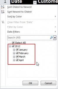
In this Excel tutorial, I respond to a viewer request. He likes the new “Roll Up Summary by Month” feature for filtering a field in an Excel 2007 – 2010 Field. What he finds frustrating – there seems to be no natural way to accomplish this with an Excel Pivot Table.

Natural Language Date Filters in Excel

Before I solve my readers dilemma, I demonstrate how to take advantage of the new “Natural Language” Date Filters that were introduced in Excel 2007. Date Filters allow you to filter records from “Today,” “Last Week,” “Next Month,” etc. They are available for Excel Tables and Excel Pivot Tables. These “Natural Language” Date Filters are a major improvement in Excel!

Group a Field for Pivot Tables

To solve my viewers question, I “Grouped” the original Date Field in his Pivot Table to produce “virtual” fields for “Month,” and “Year.” Now, it is a simple step to filter the “virtual” Month Field to obtain a “roll up” filter for individual months in the Pivot Table. Just select a single cell in the Pivot Table Date Field and choose Group Field. Make your choices in the Grouping Dialog Box and you are “good to go!”

I also show you how to take advantage of the Expand and Collapse Field Commands in a Pivot Table.

In-Depth Video Tutorial for Excel Pivot Tables

At my secure, online shopping website, you can purchase my 90-minute Video tutorial for Excel Pivot Tables. Available for immediate downloading or on a DVD-ROM. Version specific editions for Excel 2003, 2007, and 2010.

Watch Video Tutorial in High Definition

Follow this link to watch this tutorial in High Definition Mode on my YouTube Channel – DannyRocksExcels


Share and Enjoy:
  • Add to favorites
  • Facebook
  • Twitter
  • Technorati
  • Print
  • email
  • Digg
  • StumbleUpon
  • del.icio.us
  • Yahoo! Buzz
  • Google Bookmarks
  • Orkut
  • SphereIt
  • Sphinn

How to Use the Offset Function Inside a VLookup in Excel

Vlookup in Excel

VLOOKUP in Excel

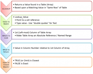
Each month, I get 5 to 6 emails of phone calls from viewers who who are having trouble using the VLOOKUP Function in Excel. In the majority of cases, the problem is that their Data Table is setup so that the “Key” field that they need to search in is NOT the Left-most or first field in the table. It is not always practical – nor desirable – to use “Cut and Paste” to rearrange the fields in the data set. So, what techniques can you use to fix this?

Use the OFFSET Function Inside a VLOOKUP Function

In this scenario, our IT Department sends us a daily report of the products that we sell including fields for the current cost and quantity on-hand. We use this report to generate additional reports and filters. This report gets saved automatically as an Excel 2010 Table with the name “Inventory.” The problem is, whenusing a VLOOKUP, that the first – or Left-most – field is NOT the “Key” field that we want VLOOKUP to use to search for a Match in order to return the current price or inventory for individual product.

The OFFSET() Function in Excel, makes it easy to reference a “starting field” that, in this case, is one column to the Right. This is perfect for our situation. We can continue to use our “named range” with the VLOOKUP!

Watch Video in High Definition

Follow this link to watch this tutorial in High Definition on my YouTube Channel – DannyRocksExcels

Visit My New Secure Online Shopping Website

I invite you to visit my new online shopping website at: http://shop.thecompanyrocks.com I have created new, extended length video tutorials that you can either purchase to download immediately or order them on a DVD-ROM. In addition, I have published versions of my 90 minute Pivot Tables Video Tutorials for Excel 2003, Excel 2007 and Excel 2010. So, I have the tutorials that you want for the Excel version that you are currently using!

Click to Play Excel Video Tutorial

Share and Enjoy:
  • Add to favorites
  • Facebook
  • Twitter
  • Technorati
  • Print
  • email
  • Digg
  • StumbleUpon
  • del.icio.us
  • Yahoo! Buzz
  • Google Bookmarks
  • Orkut
  • SphereIt
  • Sphinn

Structured Formula References in Excel 2007 and Excel 2010 – Part 2

Compare Structered References Excel 2007 v 2010

Compare Structured References 2007 v 2010

This is the second and concluding part of this series where I demonstrate how to use Structured Formula References when referring to Excel Tables.

Key Points Covered

  • The difference between Structured Formula References in Excel 2007 and Excel 2010
  • How to Edit Structured Formula References
  • How to Write Structured Formulas using the new Formula AutoComplete drop-down menu


Watch My Video Tutorial Now


Watch Video in High Definition on YouTube

Click on this link to watch this Video in High Definition on my YouTube Channel – DannyRocksExcels

Go to Part 1 in this Series of Video Tutorials

Follow this link to go to Part 1 in this Series of Tutorials about using Structured Formula References in Excel Tables.

Visit My New Secure Online Store

I have just published 6 New Products and opened a new, revised, secure online shopping website. Take a look at: http://shop.thecompanyrocks.com


Share and Enjoy:
  • Add to favorites
  • Facebook
  • Twitter
  • Technorati
  • Print
  • email
  • Digg
  • StumbleUpon
  • del.icio.us
  • Yahoo! Buzz
  • Google Bookmarks
  • Orkut
  • SphereIt
  • Sphinn

How to Use Structured Formula References for Tables in Excel 2007 and Excel 2010

Structured Formula Reference - Excel 2007

Structured Formula Reference - Excel 2007

Beginning with Excel 2007, you can – and should – convert a Standard Data Range to an Excel Table. Doing so offers several advantages:

  • You get a selection of Table Styles – including Alternate Row Shading – that make it easier to read your tables.
  • You can automatically extend the Scope of your Table – by adding additional Fields (Columns) or Records (Rows).
  • You can give your Table a “Name” to reflect the purpose of the Table.
  • You can add a Total Row to Subtotal each Field (Column) and you can change the Function used to Subtotal from a drop-down menu.
  • You can apply Structured Formula References in the Table – Enter the Formula in a Single Cell and it is Automatically copied down for each record in the Table.

“In This Row” Formula Styles

Structured Formula References use a new style of formulas. Rather than referring to a specific Cell, in an Excel Table, you refer to a Field “in this row.” This type of formula is easy to create “inside the table.” It is also fairly easy to create “outside the Table” using the new Formula AutoComplete tool. You will be using [ ] (Left & Right Brackets) for these formulas. I go over these details, in-depth, in this video tutorial.

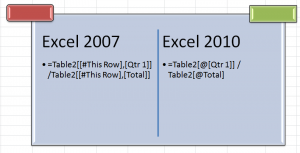
There are also distinct differences in how Structured Formula References are created between Excel 2007 and Excel 2010. These Structured Formula References are greatly streamlined in Excel 2010 – in my opinion.

The SUBTOTAL() Function and Excel Tables

I strongly recommend that you become familiar with how to use the valuable SUBTOTAL() Function in Excel when referring to the data in a Table. With the SUBTOTAL Function, you can produce a wide range of summaries anywhere on your Excel Workbook. And… the Subtotal Results reflect the totals for any “Filters” that you apply to your Table.

Play this Video in High Definition

Watch this Video in High Definition

Follow this link to watch this Excel Tutorial in High Definition on my YouTube Channel – DannyRocksExcels

Go to Part 2 in this Series of Tutorials

Follow this link to go to Part 2 in this series of tutorials about using Structured Formula References in Excel Tables.

Announcing 6 New Products on My New Online Secure Shopping Website

I invite you to visit my new online shopping site. I have added 6 new products – Extended Length Video tutorials that you can either “download now” or purchase as a DVD-ROM. Each product contains over 90 minutes of in-depth video instruction for Pivot Tables. You can choose the product to fit your version of Excel – Separate products for Excel 2003, Excel 2007 and Excel 2010.

Click here to view my new products.

Share and Enjoy:
  • Add to favorites
  • Facebook
  • Twitter
  • Technorati
  • Print
  • email
  • Digg
  • StumbleUpon
  • del.icio.us
  • Yahoo! Buzz
  • Google Bookmarks
  • Orkut
  • SphereIt
  • Sphinn

How to Create a Summary Report from an Excel Table

Functions for Executive Summary

Functions for Executive Summary

I created this Excel Video Tutorial in response to a viewer who, in her company, is not permitted to use a Pivot Table to create a report. Unfortunately, this happens more often than you might think. Nevertheless, I promised to share my tips and advice. I think that many of this tips will help Excel users at all levels.

Tips Covered in this Video Tutorial

  • Use Advanced Filter to Extract a list of unique customer names from a range with @ 4,300 records.
  • Later in the lesson, I show you how to extract this list to a different worksheet – a tip that will save you time when preparing your reports!
  • How and why to convert a normal range of data into a TABLE in Excel 2007 / 2010 or into a LIST in Excel 2003.
  • How to create “Named Ranges” for your key data cells and to use them in your Formulas and Functions.
  • How to use the SUMIF, AVERAGEIF and COUNTIF Functions in your summary report.

Keyboard Shortcuts Used in this Tutorial

  • Ctrl + T to convert to a TABLE in Excel 2007 / Excel 2010
  • Ctrl + L to convert to a LIST in EXCEL 2003
  • Ctrl + A to open up the Function Arguments Dialog Box
  • Ctrl + Shift + F3 to open the Create Names Dialog Box
  • F3 to open the Paste Names Dialog Box

I decided that I will only make this video available on YouTube – I think that you will enjoy the clarity that you get from the High-Definition / Full Screen Mode.

Watch Tutorial in High Definition on YouTube

Follow this link to view this Excel Tutorial in High Definition on my YouTubeChannel – DannyRocksExcels

Visit my new secure online shopping website

I invite you to visit http://shop.thecompanyrocks.com – my new online shopping website.

Watch Video Now

Share and Enjoy:
  • Add to favorites
  • Facebook
  • Twitter
  • Technorati
  • Print
  • email
  • Digg
  • StumbleUpon
  • del.icio.us
  • Yahoo! Buzz
  • Google Bookmarks
  • Orkut
  • SphereIt
  • Sphinn

How to Use an Excel Macro to Quickly Fill in Blank Cell Labels

Options for Filling in Blank Cell Labels

Options for Filling in Blank Cell Labels

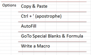
In this Excel video tutorial, I demonstrate how to write, proofreed and run a Macro that will quickly fill in values for blank cell lables in a report that you may have received from a colleague or a client.

Reports With “Holes in the Data”

Frequently, when you receive a report that was created in an Excel Pivot Table or from a relational database – e.g. MS Access – the report looks great! However, if you wish to apply filters or other analysis to this report, you will need to fill in the “missing” or blank cell labels.  

Watch This Excel Video Tutorial in High Definition

Follow this link to view this lesson in High Definition, Full Screen Mode on my YouTube Channel – DannyRocksExcels

Related Excel Video Tutorials

If you would like to learn how to convert an Excel Pivot Table to a Standard List – and to Fill in the Blank Cell Labels – click on this link to see my video tutorial on this topic.

And, here is a link to another related Excel Video Tutorial – Quickly Fill in Blank Cell Labels

Share and Enjoy:
  • Add to favorites
  • Facebook
  • Twitter
  • Technorati
  • Print
  • email
  • Digg
  • StumbleUpon
  • del.icio.us
  • Yahoo! Buzz
  • Google Bookmarks
  • Orkut
  • SphereIt
  • Sphinn

How to Take Advantage of Excel 2007 – 2010 Tables and Excel 2003 Lists

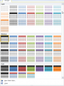
Excel Table Styles

Excel Table Styles

In this video tutorial, I cover multiple versions of Excel. I demonstrate how to take advantage of the Table Tools that were introduced in Excel 2007 and I also show you how to create Excel 2003 Lists.

Topics Covered on Video Tutorial

  • Convert a range of data to an Excel 2007, Excel 2010 Table.
  • Convert a range of data to an Excel 2003 List.
  • View and change the Total Row in each version of Excel.
  • Append new records to Tables and Lists.
  • Add a new field to Tables and Lists.
  • Write a formula in one cell of an Excel Table and have it automatically copy down for each record.
  • Change the Table Styles in Excel 2007 and 2010.
  • Use Conditional Formatting to add alternate row shading to an Excel 2003 List

Watch Video in High Definition on YouTube

Follow this link to watch this Excel Video Tutorial in High Definition on my YouTube Channel, DannyRocksExcels

Download This Excel Workbook

Click on this link to download the Excel Workbook that I used in this video tutorial.

Get my best-selling DVD-ROM, “The 50 Best Tips for Excel 2007” for only $39.95!

Share and Enjoy:
  • Add to favorites
  • Facebook
  • Twitter
  • Technorati
  • Print
  • email
  • Digg
  • StumbleUpon
  • del.icio.us
  • Yahoo! Buzz
  • Google Bookmarks
  • Orkut
  • SphereIt
  • Sphinn