Instructional Guide “9 Essential Excel 2010 Skills” – Download for Free

Instructional Guide "9 Essential Excel 2010 Skills"

Instructional Guide “9 Essential Excel 2010 Skills”

I want you to discover the scope of the Excel Training that I offer on my new video tutorial, “9 Essential Excel 2010 Skills.” So, I am offering the PDF of the Step-by-Step Instructional Guide that accompanies the video tutorial.

Link to The Company Rocks Free Resources Page

Click on this link to begin the download process for the Instructional Guide.

Instructions for Downloading the Free Instructional Guide

  1. Add this product to your secure shopping cart at my website.
  2. During Checkout, you can choose to either Register or Shop as a Guest
  3. You will need to provide a valid email address in order to receive the actual link to download my Instructional Guide.
  4. Even though you will be downloading this product, I had to set it up as a physical product with “Free Shipping.”
  5. Shortly after you complete the checkout process you will receive an email that contains a hyperlink to the file that you will download.
  6. You will be downloading a “zipped” file. So, once the download is completed, be sure to “unzip” this file!
  7. I created my Instructional Guide using the free Adobe Acrobat Reader.

Read the Instructional Guide and then Purchase my Video!

I am convinced that once you see the scope of the training in Excel 2010 that I offer, you will want to purchase the video tutorial. I offer my video in tow versions:

List of the “9 Essential Excel 2010 Skills”

9 Essential Skills for Excel 2010

9 Essential Skills for Excel 2010 Video Tutorial

These are the 9 Essential Skills that I have identified for my video tutorial:

  1. Entering Data Efficiently in Excel 2010
  2. Selecting Cell Ranges Efficiently in Excel 2010
  3. Creating and Using Named Cell Ranges in Excel 2010
  4. Applying Styles and Formatting to Excel 2010 Worksheets
  5. Working with Structured Data Sets in Excel 2010
  6. Working with Excel 2010 Formulas and Functions
  7. Using Paste Special Options in Excel 2010
  8. Using Data Validation in Excel 2010
  9. Using Excel 2010 “What-if” Analysis Tools

Excel 2010 Practice Files Included

When you purchase my video tutorial, you receive the same Excel 2010 Worksheets that I used while filming each of the 25 video tutorials. Using the same files as you view my videos, you will be able to practice your new skills. And, of course, you also receive the same Instructional Guide that I am offering for free!

I welcome your feedback! Please send me your comments via email – danny@thecompanyrocks.com – or by adding a comment below.

Thank you!


Share and Enjoy:
  • Add to favorites
  • Facebook
  • Twitter
  • Technorati
  • Print
  • email
  • Digg
  • StumbleUpon
  • del.icio.us
  • Yahoo! Buzz
  • Google Bookmarks
  • Orkut
  • SphereIt
  • Sphinn

How to Use a Check Box to “Toggle” Conditional Formatting On or Off in Excel

Sort by Color in Excel

Sort by Color in Excel

In my previous Excel Tutorial – “Conditional Formatting to Dynamically Format Dates” – I demonstrated how to  apply Conditional  Formatting based upon the number of days have passed since last contact with a customer. Now I will extend what you just learned.

Three Techniques in this Video:

  1. How to extend  Conditional Formatting Rules to additional cell ranges.
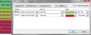
  2. How to use the “Sort by Colors” feature introduced in Excel 2007.
  3. How to add a Check Box Form Control that will “toggle” the Conditional Formatting On or Off.

Paste Special “Live Preview”

I demonstrate a great new feature introduced in Excel 2010, “Live Preview” for Paste Special. You will use Paste Special – Formats to extend the rules for Conditional Formatting to a new range of Cells

Sort by Color

Beginning with Excel 2007, you can now sort fields based upon the color of a font or a cell background. I show how this works.

The Check Box Form Control

The “key concept” to understand when using Excel’s Form Controls is the “Cell Link.” With a Check Box Control, the value in the Cell Link is TRUE when the box is “checked” while the value is FALSE when it is Unchecked. We can use this information to create a “Conditional Format based upon a Formula.”

Conditional Formatting Rules

When you base Conditional Formatting upon a Formula, the result of that formula must return TRUE in order apply this formatting. Setting the background cell color to “White” effectively “hides” the previous background cell colors.

Shop for The 50 Best Tips for Excel 2007

Shop for The 50 Best Tips for Excel 2007

Resources Offered for Sale

I encourage you to visit my secure online shopping website – http://shop.thecompanyrocks.com – to preview the many training resources that I offer you. Check out my latest Excel Training Videos:

Watch this Video in High Definition

Click on this link to watch this video in High Definition on my YouTube Channel – DannyRocksExcels


Share and Enjoy:
  • Add to favorites
  • Facebook
  • Twitter
  • Technorati
  • Print
  • email
  • Digg
  • StumbleUpon
  • del.icio.us
  • Yahoo! Buzz
  • Google Bookmarks
  • Orkut
  • SphereIt
  • Sphinn

How to Dynamically Color-Code Dates with Conditional Formatting in Excel

Conditional Formatting for Dates

Conditional Formatting for Dates

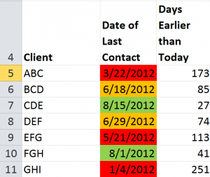
One of my viewers wants to learn how to “dynamically” color-code cells that contain dates. She is monitoring the frequency of contact with her clients and she wants Excel to automatically apply:

  • One background color to cells where it has been less than 60 days since last contact
  • A different color when the time frame is between 60 and 90 days
  • A third color when it has been over 90 days since the last contact with a client

Here, I demonstrate how she can do this using Conditional Formatting Rules. However, this will only work if you are using Excel 2007 or Excel 2010.

Understanding Dynamic Date Functions

In order to make this visualization “dynamic,” I make references to cells that contain the =TODAY() Function. This is a “volatile” function that updates automatically based upon the date in your computer system’s clock. I use this to classify the last date of contact with her clients.

Improvements in Conditional Formatting

Beginning with Excel 2007, you can now apply multiple rules that use formulas. Remember that when you use a formula, it must evaluate as “TRUE” in order to apply the formatting that you specify.

Formulas Used to Apply Conditional Formatting

Conditional Formatting Rules

Rules for Conditional Formatting

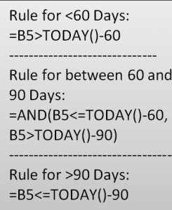
To make it easier for you to practice this skill, I have posted this table that details the formulas that I used for each of the three rules in my video tutorial.Note that with the middle condition, I use the =AND() Function. All logical tests must answer TRUE for the AND() Function to return TRUE.

It will take a little bit of practice for you to become comfortable with these formulas. As a Best Practice, I recommend that you create a table of formulas so that you can see how a “tweak” in your formula can turn a FALSE answer into a TRUE answer.

Related Video

Follow this link to Part Two in this Series. I demonstrate how to “toggle” Conditional Formatting On or Off by using a Check Box Control in Excel.

Watch this Video in High Definition

Follow this link to watch my Excel Tutorial in High Definition on my YouTube Channel – DannyRocksExcels

Get the Best Tips and Training for Excel

Click on this link to learn more about my best-selling DVD-ROM, “The 50 Best Tips for Excel 2007.” This link will take you to my secure online shopping website –  http://shop.thecompanyrocks.com

Subscribe to my Video Podcast on iTunes

Here is the link to go to my free Video Podcast, “Danny Rocks Tips and Timesavers” on iTunes.


Share and Enjoy:
  • Add to favorites
  • Facebook
  • Twitter
  • Technorati
  • Print
  • email
  • Digg
  • StumbleUpon
  • del.icio.us
  • Yahoo! Buzz
  • Google Bookmarks
  • Orkut
  • SphereIt
  • Sphinn

How to Highlight Different Values in a Row with Excel’s Go To Special

Go To Special Dialog Box

Go To Special – Row Differences

I have published several video tutorials on the topic of Highlighting and Deleting Duplicate Records in Excel. However, a viewer recently asked me how to highlight cells that contain different values in the same Row. This is not as “crazy” as it first seems.

Scenario for this Tutorial

I am trying to determine accurate inventory counts for my product line. I have the count that the computer shows. I also have records from three different auditors who have performed manual counts. I need to easily highlight the cells where the inventory count “is off.” That is where there is a discrepancy between what the computer shows and what a manual count shows.

Go To Special Dialog Box

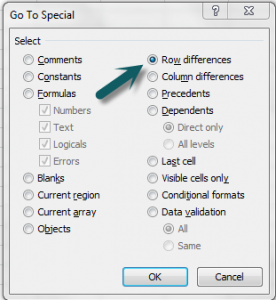
The commands in the Go To Special Dialog Box are some of my favorite tools. In my experience, I have found that most Excel users have never explored this dialog box.  I think that will change after you watch this video tutorial. For the Row Differences tool, you first select the range of cells that contain your data – beginning with the left-most column. The Row Differences will use this left-most column as the “baseline” and highlight each cell in that row that contains a value that is different from this baseline.

Sorting & Filtering by Color

Beginning with Excel 2007, you can Sort by Color and you can also Filter by Color. After the cells were highlighted with the Row Differences command, I applied a background cell color to each highlighted cell.

Use one of my favorite Keyboard Shortcuts, Ctrl + Shift + L, when working with Filters in Excel 2007 or Excel 2010.

Watch this Excel Tutorial in High Definition

You can watch this tutorial in High Definition on my YouTube Channel – DannyRocksExcels.  Click on this link to watch this video now.

Video Tutorials for Highlighting Duplicate Records

I mentioned that I have published many Excel Tutorials on the Topic of Highlighting & Removing Duplicate Records. Here are links to my tutorials:

Shop for Excel Training Resources

I invite you to visit my secure online shopping website – http://shop.thecompanyrocks.com – to examine and purchase the many training resources that I offer.

Watch My Video Podcasts on iTunes

Click on this link to watch my “Danny Rocks Tips and Timesavers” video podcast on iTunes. – It is free of charge!

 Note: The original Podcast Video did not have the correct video settings. This video has now been updated.


Share and Enjoy:
  • Add to favorites
  • Facebook
  • Twitter
  • Technorati
  • Print
  • email
  • Digg
  • StumbleUpon
  • del.icio.us
  • Yahoo! Buzz
  • Google Bookmarks
  • Orkut
  • SphereIt
  • Sphinn

How to Add Summary Information for Excel Workbook Properties

Almost everyone has experienced the frustration of being unable to locate an Excel Workbook on their computer. You can’t remember the name or the location of the Workbook. You waste valuable time searching in vain.

Tags for Document Search

Tags for Document Search

One way to minimize this frustration is to add Excel Workbook Properties that Summarize the content and purpose of the document. By adding Tags, Keywords, Client Names or Project Titles in the Properties Summary you make it easier for your computer to Index and Find your documents.

Fortunately, beginning with Microsoft Office 2007, it is a lot easier to add these properties to an Excel Workbook. In this video tutorial, I show you how to do this.

Displaying Recent Documents

Did you know that you can display up to 50 Recent Documents? Even better, you can “Pin” important documents so that they remain on the list. This is a valuable tool when you need to access important files, for example, once a month! I show you how to do this on the video.

Shop for Additional Resources

I invite you to visit my secure online shopping website – http://shop.thecompanyrocks.com – where you can purchase all of the training materials that I have developed.

Watch Video in High Definition

Click on this link to watch my Excel Tutorial in High Definition on my YouTube Channel – DannyRocksExcels

Watch this Video Now


Share and Enjoy:
  • Add to favorites
  • Facebook
  • Twitter
  • Technorati
  • Print
  • email
  • Digg
  • StumbleUpon
  • del.icio.us
  • Yahoo! Buzz
  • Google Bookmarks
  • Orkut
  • SphereIt
  • Sphinn

How to SUM Values in One Field Based on Criteria from Multiple Fields in Excel

SUMIFS and DSUM Functions

SUMIFS and DSUM Functions

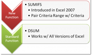
The new SUMIFS() Function was introduced in Excel 2007. With SUMIFS, you can sum the values in one field based up criteria that comes from multiple fields. This is a very valuable Function.

SUMIFS Function

The key to understanding SUMIFS, is that you “pair” a criteria range with the criteria for that range. As you watch my tutorial, the importance of this concept will become clear to you.

DSUM Function

If you are using – or need to create workbooks that are compatible with – older versions of Excel – e.g. Excel 2003, you can use the DSUM Function to achieve the same results. The DSUM belongs to the Database Functions set in Excel.

Use Named Cell Ranges in Formulas

I highly recommend that you learn how to create – and then use – named cell references in your Excel Formulas and Functions. In this tutorial, I show you how to do this. Once you have created a named cell reference, you can use the F3 Keyboard Shortcut to show a dialog box that lists all of the named Ranges that you can post into your formulas. This will save you time and help to ensure accuracy in your formulas – especially when you cop a formula to another location.

Bonus: Create Drop-down Menu with Data Validation

When using Multiple Criteria, I like to be able to select my criteria values from a drop-down list. In this lesson, I demonstrate how to do this using Data Validation in Excel.

Learn More Excel Tips

I invite you to visit my new, secure, online shopping website – http://shop.thecompanyrocks.com. Here, you can learn more about the tips on my best-selling DVD-ROM, “The 50 Best Tips for Excel 2007.”


Watch Video in High Definition

Here is the link to view this Excel Tutorial in High Definition on my YouTube Channel – DannyRocksExcels

YouTube Video

Share and Enjoy:
  • Add to favorites
  • Facebook
  • Twitter
  • Technorati
  • Print
  • email
  • Digg
  • StumbleUpon
  • del.icio.us
  • Yahoo! Buzz
  • Google Bookmarks
  • Orkut
  • SphereIt
  • Sphinn

Structured Formula References in Excel 2007 and Excel 2010 – Part 2

Compare Structered References Excel 2007 v 2010

Compare Structured References 2007 v 2010

This is the second and concluding part of this series where I demonstrate how to use Structured Formula References when referring to Excel Tables.

Key Points Covered

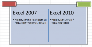
  • The difference between Structured Formula References in Excel 2007 and Excel 2010
  • How to Edit Structured Formula References
  • How to Write Structured Formulas using the new Formula AutoComplete drop-down menu


Watch My Video Tutorial Now


Watch Video in High Definition on YouTube

Click on this link to watch this Video in High Definition on my YouTube Channel – DannyRocksExcels

Go to Part 1 in this Series of Video Tutorials

Follow this link to go to Part 1 in this Series of Tutorials about using Structured Formula References in Excel Tables.

Visit My New Secure Online Store

I have just published 6 New Products and opened a new, revised, secure online shopping website. Take a look at: http://shop.thecompanyrocks.com


Share and Enjoy:
  • Add to favorites
  • Facebook
  • Twitter
  • Technorati
  • Print
  • email
  • Digg
  • StumbleUpon
  • del.icio.us
  • Yahoo! Buzz
  • Google Bookmarks
  • Orkut
  • SphereIt
  • Sphinn

Use the Show Values As Formulas in Excel Pivot Tables

Show Values As

Show Values As in Pivot Table

I participate in a number of Group Discussion Boards on LinkedIn. In this video tutorial, I address one question that was recently asked:

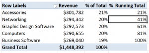
“Is it possible to show a Percentage of Running Total formula in a Pivot Table?”

The answer is, “Yes, if you are using Excel 2010. If you are using earlier versions of Excel, you can use a work-around outside the Pivot Table.”

New in Excel 2010

A great new feature introduced in Excel 2010 is the drop-down menu for the “Show Values As’ in a Pivot Table Calculation. In earlier versions of Excel, the Show Values As option was not so obvious. And, I found that many of my clients did not know how to use it – or could not locate the drop-down menu.

Work-Around for Show % of Running Total

While the “Running Total in…” calculation has been available for quite some time, the “% of Running Total in …” formula is brand new in Excel 2010. The work-around that I demonstrate is to first, create the Show As “Running Total in …” formula. Then change the Font and background of these cells to “White.” Next, write a standard formula “outside of the Pivot Table” that references these cells. Be sure to turn off the “GetPivotData” Formula when you write this formula.

Download Extended Length Pivot Table Video Tutorials

Click on this link to learn about my new “extended length” video tutorials for Pivot Tables. They are availabe for Excel 2003, Excel 2007 and Excel 2010.

Watch Video in High Definition on YouTube

Follow this link to watch this video in High Definition on my YouTube Channel – DannyRocksExcels

Master Excel Pivot Tables in 90 Minutes

Follow this link to learn about my new “Extended Length” – 90 Minutes – Video Tutorials


Share and Enjoy:
  • Add to favorites
  • Facebook
  • Twitter
  • Technorati
  • Print
  • email
  • Digg
  • StumbleUpon
  • del.icio.us
  • Yahoo! Buzz
  • Google Bookmarks
  • Orkut
  • SphereIt
  • Sphinn

Create a Pivot Chart to Present a Frequency Distribution Report

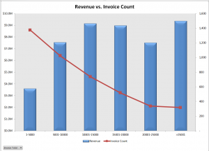
Combination Chart for Frequency Report

Quite a few of my viewers requested that I continue my series of creating and presenting a “Frequency Distribution Report” using an Excel Pivot Table. So, here is the new Part 3 in the series!

In this Excel Video Tutorial, I demonstrate – using Excel 2010 – how to create a Pivot Chart for the Frequency Distribution Pivot Table that I created and modified in Parts 1 and 2 of this series.

Key Point: A Pivot Chart Must be based on a Pivot Table Report!

  • Any structural changes that you make to the Pivot Table are reflected in the Pivot Chart.
  • If you “filter” the Pivot Chart, those filters apply to the Pivot Table that is the basis for your Pivot Chart – and vice versa.

Focus on the Chart

As I demonstrate in this video – posted on YouTube – I prefer to focus on one task at a time. I prefer to get the formatting and structure of the Chart “right” before I think about using Filers and other “goodies to add .” This “Best Practice” helps me to get more accomplished in less time!

My bottom line is: “Focus on the task at hand. Eliminate any possible distractions from that primary task!”

A correctly designed Pivot Chart will help you to present your information accurately and interactively! For this presentation, I decided that a “Combination Chart” would be the best way to present the information that I wanted to convey. A “Combination Chart” allows you to have a Primary Axis (Revenue) that uses a Column Chart Type and a Secondary Axis (Invoice Count) that uses a Line Chart Type.

When to Use a Secondary Chart Axis

In this example, there is a wide difference between the two fields that we are charting:

  • Revenue for the Invoices in the “Bin Range” is in “the millions!
  • Count of Invoices in the “Bin Range” falls into the hundreds and low thousands.

Using a “Combination Chart” in this example – (Column Chart for Revenue in Millions) and Count of Invoices (Line Chart for Count in Hundreds) allows you to present the “relationship” between both metrics. I show you step-by-step how to create this combination chart!


Watch This Video in High Definition on YouTube

Follow this link to view this video tutorial in High Definition on my YouTube Channel – DannyRocksExcels

Click this link to view Part 1 of the 3 Part series – Creating a Frequency Distribution  Report with Excel Pivot Table

Click this link to view Part 2 of the 3 Part series – Formatting a Frequency Distribution Report with Excel Pivot Table

Share and Enjoy:
  • Add to favorites
  • Facebook
  • Twitter
  • Technorati
  • Print
  • email
  • Digg
  • StumbleUpon
  • del.icio.us
  • Yahoo! Buzz
  • Google Bookmarks
  • Orkut
  • SphereIt
  • Sphinn

How to Take Advantage of Excel 2007 – 2010 Tables and Excel 2003 Lists

Excel Table Styles

Excel Table Styles

In this video tutorial, I cover multiple versions of Excel. I demonstrate how to take advantage of the Table Tools that were introduced in Excel 2007 and I also show you how to create Excel 2003 Lists.

Topics Covered on Video Tutorial

  • Convert a range of data to an Excel 2007, Excel 2010 Table.
  • Convert a range of data to an Excel 2003 List.
  • View and change the Total Row in each version of Excel.
  • Append new records to Tables and Lists.
  • Add a new field to Tables and Lists.
  • Write a formula in one cell of an Excel Table and have it automatically copy down for each record.
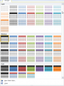
  • Change the Table Styles in Excel 2007 and 2010.
  • Use Conditional Formatting to add alternate row shading to an Excel 2003 List

Watch Video in High Definition on YouTube

Follow this link to watch this Excel Video Tutorial in High Definition on my YouTube Channel, DannyRocksExcels

Download This Excel Workbook

Click on this link to download the Excel Workbook that I used in this video tutorial.

Get my best-selling DVD-ROM, “The 50 Best Tips for Excel 2007” for only $39.95!

Share and Enjoy:
  • Add to favorites
  • Facebook
  • Twitter
  • Technorati
  • Print
  • email
  • Digg
  • StumbleUpon
  • del.icio.us
  • Yahoo! Buzz
  • Google Bookmarks
  • Orkut
  • SphereIt
  • Sphinn