COUNTIF And SUMIF Functions | The Company Rocks

Danny October 2, 2012 Leave a Comment

The 10 Most Watched Excel YouTube Videos for September 2012

My YouTube Channel – DannyRocksExcels – had 141,586 individual views during the month of September 2012:

Here is a list – with Hyperlinks – to the 10 Most Watched Excel Videos

Thanks to my 4,500 Subscriber on YouTube!

I extend my heartfelt thanks to my many loyal viewers and subscribers to my Excel video tutorials. Your feedback and requests for solutions have formed the foundation for my Excel Training Videos.

9 Essential Excel 2010 Skills

Learn More About my Extended Length Excel Video Training Resources

I have created a series of Extended Length Video Training Resources in the category of “Master Excel in Minutes.” I invite you to follow this link to learn more about my new series of videos.

Share and Enjoy:

Filed Under: COUNTIF and SUMIF Functions, Excel Data Tables and Lists, Excel Forms, Excel Formulas, Excel Functions, Excel Training, Lookup Functions in Excel, Most Viewed Excel Videos, Pivot Tables, SUMIF and SUMIFS Functions, Workbooks and Worksheets in Excel, YouTube Videos by Danny Rocks Tagged: "What-if" Analysis in Excel, Excel Pivot Charts, Excel Pivot Tables, Excel Video Training, Solver Tool in Excel, Video lessons for Excel

Danny September 20, 2012 Leave a Comment

Instructional Guide “9 Essential Excel 2010 Skills” – Download for Free

Instructional Guide “9 Essential Excel 2010 Skills”

I want you to discover the scope of the Excel Training that I offer on my new video tutorial, “9 Essential Excel 2010 Skills.” So, I am offering the PDF of the Step-by-Step Instructional Guide that accompanies the video tutorial.

Link to The Company Rocks Free Resources Page

Click on this link to begin the download process for the Instructional Guide.

Instructions for Downloading the Free Instructional Guide

Add this product to your secure shopping cart at my website.
During Checkout, you can choose to either Register or Shop as a Guest
You will need to provide a valid email address in order to receive the actual link to download my Instructional Guide.
Even though you will be downloading this product, I had to set it up as a physical product with “Free Shipping.”
Shortly after you complete the checkout process you will receive an email that contains a hyperlink to the file that you will download.
You will be downloading a “zipped” file. So, once the download is completed, be sure to “unzip” this file!
I created my Instructional Guide using the free Adobe Acrobat Reader.

Read the Instructional Guide and then Purchase my Video!

I am convinced that once you see the scope of the training in Excel 2010 that I offer, you will want to purchase the video tutorial. I offer my video in tow versions:

List of the “9 Essential Excel 2010 Skills”

9 Essential Skills for Excel 2010 Video Tutorial

These are the 9 Essential Skills that I have identified for my video tutorial:

Entering Data Efficiently in Excel 2010
Selecting Cell Ranges Efficiently in Excel 2010
Creating and Using Named Cell Ranges in Excel 2010
Applying Styles and Formatting to Excel 2010 Worksheets
Working with Structured Data Sets in Excel 2010
Working with Excel 2010 Formulas and Functions
Using Paste Special Options in Excel 2010
Using Data Validation in Excel 2010
Using Excel 2010 “What-if” Analysis Tools

Excel 2010 Practice Files Included

When you purchase my video tutorial, you receive the same Excel 2010 Worksheets that I used while filming each of the 25 video tutorials. Using the same files as you view my videos, you will be able to practice your new skills. And, of course, you also receive the same Instructional Guide that I am offering for free!

I welcome your feedback! Please send me your comments via email – danny@thecompanyrocks.com – or by adding a comment below.

Thank you!

Share and Enjoy:

Filed Under: COUNTIF and SUMIF Functions, Data Validation, Everyday Calculations in Excel, Excel Basics, Excel Data Tables and Lists, Excel Formulas, Excel Functions, Excel Training, Format Cells in Excel, Goal Seek in Excel, MS Excel Tips, MS Excel Training, Names for Cells and Ranges, New in Excel 2010, Online Store for The Company Rocks, Subtotals and Outlines in Excel, SUMIF and SUMIFS Functions, Video Training Courses, What-if Analysis Tagged: "What-if" Analysis in Excel, Absolute cell reference, AutoFill Options, COUNTIF Function, Create Subtotals in Excel, Data Validation, Excel Functions, Excel Video Training, Go To Special dialog box, IF() Function, Keyboard Shortcuts in Excel, Learn to use AutoFill in Excel, Lookup Functions in Excel, Named Cell in a formula, Paste Special, SUMIF Function, Video lessons for Excel, VLOOKUP Function

Danny September 19, 2011 2 Comments

How to Create a Summary Report from an Excel Table

Functions for Executive Summary

I created this Excel Video Tutorial in response to a viewer who, in her company, is not permitted to use a Pivot Table to create a report. Unfortunately, this happens more often than you might think. Nevertheless, I promised to share my tips and advice. I think that many of this tips will help Excel users at all levels.

Tips Covered in this Video Tutorial

Use Advanced Filter to Extract a list of unique customer names from a range with @ 4,300 records.
Later in the lesson, I show you how to extract this list to a different worksheet – a tip that will save you time when preparing your reports!
How and why to convert a normal range of data into a TABLE in Excel 2007 / 2010 or into a LIST in Excel 2003.
How to create “Named Ranges” for your key data cells and to use them in your Formulas and Functions.
How to use the SUMIF, AVERAGEIF and COUNTIF Functions in your summary report.

Keyboard Shortcuts Used in this Tutorial

Ctrl + T to convert to a TABLE in Excel 2007 / Excel 2010
Ctrl + L to convert to a LIST in EXCEL 2003
Ctrl + A to open up the Function Arguments Dialog Box
Ctrl + Shift + F3 to open the Create Names Dialog Box
F3 to open the Paste Names Dialog Box

I decided that I will only make this video available on YouTube – I think that you will enjoy the clarity that you get from the High-Definition / Full Screen Mode.

Watch Tutorial in High Definition on YouTube

Follow this link to view this Excel Tutorial in High Definition on my YouTubeChannel – DannyRocksExcels

Visit my new secure online shopping website

I invite you to visit http://shop.thecompanyrocks.com – my new online shopping website.

Watch Video Now

Share and Enjoy:

Filed Under: COUNTIF and SUMIF Functions, Excel Data Tables and Lists, Excel Functions, Excel Training, Keyboard Shortcuts, Names for Cells and Ranges, YouTube Videos by Danny Rocks Tagged: Advanced Filter for Excel data, AverageIf Function in Excel, COUNTIF Function, Excel 2007 Tables, Excel 2010 Tables, Excel Keyboard Shortcuts, Excel Video Training, Lookup Functions in Excel, Named Cells and Ranges, SUMIF Function, Video lessons for Excel

Danny September 15, 2011 1 Comment

How to Identify and Then Delete Duplicate Records in Excel

Identify & Delete Duplicates

It is almost inevitable that, over time, your Excel data set will contain duplicate records. This can be costly – if the duplicate records are in your mailing list. And it can also result in errors when you count and calculate data.

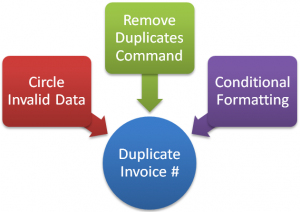
Three Methods to Identify and Delete Duplicate Records

In this Excel Tutorial, I demonstrate three approaches to identify duplicate records in a data set:

Circle Invalid Data – This tool works in coordination with Data Validation.
Remove Duplicates – This powerful command was introduced in Excel 2007. It does not “preview” the records to be deleted, so my advice is to use this command with a copy of your data.
Conditional Formatting – Greatly improved for Excel 2007 and Excel 2010. Now, you have a menu choice to apply conditional formatting to either Duplicate or Unique Records. If you are still using Excel 2003 or earlier, I show you how to write the formula needed to use Conditional Formatting to highlight duplicate records.

Watch The Tutorial in High Definition on YouTube

Follow this link to view this Excel Tutorial in High Definition on my YouTube Channel – DannyRocksExcels

Share and Enjoy:

Filed Under: Conditional Formatting, COUNTIF and SUMIF Functions, Data Validation, Excel Training, New in Excel 2007, YouTube Videos by Danny Rocks Tagged: Circle Invalid Data in Excel, Conditional formatting in Excel, COUNTIF Function, Custom Data Validation Formulas, Data Validation, Excel Video Training, Logical Formuls, Remove Duplicates in Excel, Video lessons for Excel

Danny September 8, 2011 1 Comment

How to Prevent Duplicate Entries in Excel with Data Validation

Formula for Data Validation

Over time, it is easy for duplicate entries to creep into an Excel Data Set. In this video tutorial, I show you, step-by-step, how to apply Data Validation to a range of cells so that anyone who attempts to enter a duplicate value will be prevented from doing so.

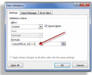
Use a “Logical Formula” for Data Validation

In this lesson, I show you how to “customize” the COUNTIF Function in the Data Validation Dialog Box so that it returns the value of TRUE. Logical formulas return either TRUE or FALSE. You MUST use a Logical Formula in Data Validation.

What Else is Covered in this Tutorial?

Use Paste Special – Validation to extend Data Validation to a wider range of cells
Use Find – Go to Special – Validation to highlight all cells on worksheet that contain Data Validation
Use Circle Invalid Entries from the Data Validation menu to automatically “draw a red circle” around existing cells that contain duplicate values
How to quickly remove Data Validation from a Range of Cells

Watch Tutorial in High Definition

Follow this link to my YouTube channel – DannyRocksExcels – where you can watch this tutorial in High Definition mode.

Share and Enjoy:

How to Prevent Duplicate Entries in Excel with Data Validation [ 10:23 ] Play Now | Play in Popup | Download (1824)

Filed Under: COUNTIF and SUMIF Functions, Data Validation, Excel Training, Podcast Tips & Timesavers Tagged: COUNTIF Function, Data Validation, Excel Video Training, Prevent duplicate entries, Remove Duplicate Entries, Show duplicate records, Video lessons for Excel

Danny January 30, 2011 3 Comments

How to Use Conditional Formatting to Compare Two Excel Lists

Clients and viewers frequently ask me to help them to compare two differeny lists in Excel. They want to find – or highlight – the values that are different in each list. For example, which customers appear in the 1st list but NOT in the 2nd list. So, I created this video lesson to demonstrate how to do this with Conditional Formatting.

In an earlier Excel Video Lesson, I demonstrated how to compare two Excel lists using either the MATCH() Function or the VLOOKUP() Function.

Conditional Formatting Rule

Use Conditional Formatting

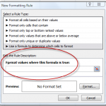
I demonstrate how to use Conditional Formatting to Highlight the Cell Values that are different when you compare two Excel Lists. I will use a “New Rule with a Formula” that must return the answer TRUE, to trigger the special formatting.

In Conditional Formatting, you first establish a “condition” that can be answered as either TRUE or FALSE. Then, for those cells where the answer to the condition is TRUE. the special “cell formatting” that you chose will apply.

In this lesson we will be using this Formula: =COUNTIF(List 2, 1st cell in List 1) = 0.

Steps to follow:

Select the cells that you want the Conditional Formatting to apply to- in our example List 1.
On the Home Tab of the Ribbon, click the Conditional Formatting arrow and select New Rule.
Select New Rule – “Use a Formula to determine which cells to format.”
Enter the formula – e.g. =COUNTIF(Range, Criteria) = 0 where the “Range” is the list of values in List 2 (Absolute Reference) and the “Criteria” is the 1st cell reference in List 1 (Relative Reference).
Choose the Format for the cells when the condition is met – the result is TRUE. In this example, I choose to “FILL” the cells with a Blue background color.

Want to watch this video in High Definition, Full-Screen Mode? Click here to go to my YouTube Channel, DannyRocksExcels

Learn to “Master Excel in Minutes – Not Months!”

Share and Enjoy:

How to Use Conditional Formatting to Compare Two Excel Lists [ 8:33 ] Play Now | Play in Popup | Download (1495)

Filed Under: Conditional Formatting, COUNTIF and SUMIF Functions, Excel Formulas, Excel Training, Podcast Tips & Timesavers Tagged: Absolute cell reference, Compare lists in Excel, Conditional formatting in Excel, COUNTIF Function, Excel Functions, Excel Video Training, Lookup Functions in Excel, MATCH() Function in Excel, Named Cell in a formula, Video lessons for Excel, VLOOKUP Function

Danny October 16, 2010 Leave a Comment

How to Add a Check Box Control to an Excel Form

Judging by the comments that I get from many clients, adding a “Check Box Control” to and Excel Form is not as easy as it appears at first glance.

And, I agree! I, too, struggled with adding Form Controls in Excel. Most of the explanations that I read seemed to add more confusion than clarification!

Spin Button Controls

That is why I created this Excel Training Video: to lead you through the process; to save you some time and to ease your frustration.

Key Points to Remember:

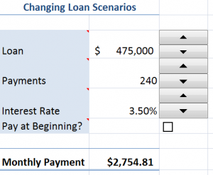
In Excel 2007, be sure to display the “Developer Tab” on the Ribbon in order to to Insert any Form Control.
Choose the Controls in the “Forms Controls” and NOT in the Active X Controls.
After you “draw” the Control Box on your Form, be sure to select a “Cell Link” to enable the Check Box Control.
Remember that a Check Box Control can only be applied when the result of the Formula or Option is a Logical Value – either a result of “True or False.”

Don’t be scared off! I find that this is an Excel concept that is better presented “visually.” I struggled for some time when I “read” how to add form controls.

So … I welcome your thoughts – “True or False.” Did I make this easy for you to understand?

Please feel free to add your comments below!

Watch My Video on YouTube

Follow this link to watch my tutorial on my YouTube Channel – DannyRocksExcels

Watch Video Now

Master Excel in Minutes Training Resources

I have created a series of extended length Excel Training Videos. I invite you to visit my secure online shopping site to:

Learn how to “Master Excel in Minutes – Not Months!”

Share and Enjoy:

How to Add a Check Box Control to an Excel Form [ 10:15 ] Play Now | Play in Popup | Download (1315)

Filed Under: COUNTIF and SUMIF Functions, Excel Forms, Excel Training, Most Viewed Excel Videos, Podcast Tips & Timesavers, YouTube Videos by Danny Rocks Tagged: Cell Link in Excel Forms, Conditional formatting in Excel, Excel Form Controls, Excel Forms, Excel Formulas, Excel Video Training, PMT() Function, Tips and Time Savers, Video lessons for Excel

Danny September 12, 2010 Leave a Comment

Prevent Duplicate Cell Entries with Excel Data Validation

Unfortunately, it is much too easy for a data entry clerk to assign duplicate account numbers. And this is a disaster waiting to happen. To prevent this from happening, use Excel’s Data Validation tool. In this short video lesson, I show you how to use the =COUNTIF() function in the Data Validation dialog box to ensure that only unique account numbers can be assigned to your customers.

I also show you how to extend the range of cells that contain this data validation rule: You use the Paste Special – Validation command.

This is one of “The 50 Best Tips for Excel 2007.” Click here to purchase the DVD using my secure shopping cart.

Learn how to “Master Excel in Minutes – Not Months!”

Share and Enjoy:

Use Data Validation to Prevent Duplicate Entries [ 5:38 ] Play Now | Play in Popup | Download (761)

Filed Under: COUNTIF and SUMIF Functions, Excel Training, Podcast Tips & Timesavers Tagged: COUNTIF Function, Data Validation, Excel Video Training, MS Excel Training, Paste Special, Tips and Time Savers, Video lessons for Excel

Danny July 8, 2010 1 Comment

Two Ways to Produce an Executive Summary of an Excel List

On one of the technology blogs that I follow, there is a debate over the best way to produce an Executive Summary of the information in an Excel Data List. Some people like the idea of using Excel’s =SUMIF() Function for this while others recommend creating a Pivot Table as the summary.

You decide – after watching this short video demonstration using both approaches. And, add a comment or drop me an email to let me know your thoughts.

This Excel Video Lesson is available for you to download as a Podcast on iTunes.

Follow this link to go to the “Danny Rocks Tips and Timesavers” podcast.

Learn how to “Master Excel in Minutes – Not Months!”

Share and Enjoy:

Summarize Excel Data with SUMIF Function or Create a Pivot Table [ 5:10 ] Play Now | Play in Popup | Download (1088)

Filed Under: COUNTIF and SUMIF Functions, Excel Training, Pivot Tables, Podcast Tips & Timesavers, Video Training Courses Tagged: Excel Datalist, Excel Keyboard Shortcuts, Excel Pivot Tables, Excel Video Training, Executive Summary in Excel, MS Excel Training, Named Cell in a formula, Named Ranges in Excel, SUMIF Function, Tips and Time Savers, Video lessons for Excel

Danny May 15, 2010 Leave a Comment

I Have Updated My Index of Excel Video Lessons

As part of the process of reorganizing my website, I have updated my “Index of Excel Video Lessons” page. The content of this page will be updated as I add each new Excel Video Training Lesson. So, I suggest that you click here to go to the Video Index and then save the page as one of your “Favorites” if you want to learn how to really get the most out of Excel or to find a quick answer when you are using Excel.

On the Index Page you can see an organized listing of my Excel Videos by Category – e.g. Formulas, Formatting, Pivot Tables “What-if” Analysis, etc. Each lesson is “hyperlinked” so that you can just click on the topic to go directly to the lesson that you are interested in.

I indicate in the title if the lesson is specific to Excel 2007. All my new Excel video lessons are created using Excel 2007.

If there is a topic that you would like me to cover, send me an e-mail message – danny@thecompanyrocks.com

If you enjoy my video instruction, I encourage you to purchase my DVD, “The 50 Best Tips for Excel 2007.” The DVD contains over 5 1/2 hours of Tips, Tricks & Techniques to help you to master the program – and to save a considerable amount of time while working in Excel! Click here to enter my secure shopping site.

Thank you for your support and encouragement!

Danny Rocks

Share and Enjoy:

Filed Under: COUNTIF and SUMIF Functions, Everyday Calculations in Excel, Excel Basics, Excel Data Tables and Lists, Excel Date and Time Functions, Excel Financial Tools, Excel Formulas, Excel Functions, Excel Training, Import Data into Excel, Lookup Functions in Excel, MS Excel 2007 DVD, MS Excel Tips, MS Excel Training, Online Store for The Company Rocks, Pivot Tables, Text Functions, Tips and Time Savers, Training, Video Training Courses, What-if Analysis Tagged: Excel Video Training, MS Excel Training, Tips and Time Savers, Video lessons for Excel

Danny Rocks “Training You to Excel”

Follow Danny on Social Media

Top 10 YouTube Excel Videos

Thanks to my 4,500 Subscriber on YouTube!

Learn More About my Extended Length Excel Video Training Resources

Link to The Company Rocks Free Resources Page

Instructions for Downloading the Free Instructional Guide

Read the Instructional Guide and then Purchase my Video!

List of the “9 Essential Excel 2010 Skills”

Excel 2010 Practice Files Included

Tips Covered in this Video Tutorial

Keyboard Shortcuts Used in this Tutorial

Watch Tutorial in High Definition on YouTube

Visit my new secure online shopping website

Watch Video Now

Three Methods to Identify and Delete Duplicate Records

Watch The Tutorial in High Definition on YouTube

Use a “Logical Formula” for Data Validation

What Else is Covered in this Tutorial?

Related Topic – Conditional Formatting in Excel

Watch Tutorial in High Definition

Use Conditional Formatting

Steps to follow:

Key Points to Remember:

Watch My Video on YouTube

Watch Video Now

Master Excel in Minutes Training Resources

Locate My Video Tutorials by Category

Seach My Website with Keywords

Podcast Feeds

Blogroll

Blogs for Business Writing

Blogs for Excel

Blogs for Presentations

Register or Log In

Tags