Three and a Half Ways to Average Excel Data Using Criteria

AverageIf Function in Excel

AverageIf Function in Excel

It is easy to use Excel’s AVERAGE Function to get the average for an entire range of data. But, what if you are asked to produce a report that shows the average for select groups of records – for example, average test results for the female students only; or for the male students only? What approach do you take? What Functions do you use to produce this report?

Three and a Half Ways to Produce this Report

  • SUBTOTALS – Easy to use. Remember to sort your data first using the field that you want to subtotal.
  • AVERAGEIF Function – Very easy to use. Only works in Excel 2007 and Excel 2010.
  • DAVERAGE Function – Will work in any version of Excel. Easy to add or change the Criteria.
  • PIVOT TABLE – Very easy to create. No need to write a formula. Create report with @ 6 mouse clicks!

My Preferred Approach – Create a Pivot Table Report

While Pivot Tables are the most powerful tool in Excel, they are also one of the easiest tools to use in Excel! Why?

  • Because you can create a Pivot Table Report without writing a single formula!
  • You can create this Pivot Table Report with about six clicks of the mouse.
  • You cannot possibly harm your underlying data when you create Pivot Tables!

Download a One Hour- Plus / In-depth Video Tutorial on Pivot Tables – for $9.95

I have created a series of Excel Video Tutorials that you can download for $9.95 US Dollars each. Here is a link to my informational page that gives you the details.

  • Are you Using Excel 2003? – I created a video recording for Pivot Tables using Excel 2003 that you can download for $9.95!
  • Are you Using Excel 2007? – I created a video recording for Pivot Tables using Excel 2007 that you can download for $9.95!
  • Are you Using Excel 2010? – I created a video recording for Pivot Tables using Excel 2010 that you can download for $9.95!

As with all of my products, I guarantee that you will be 100% Satisfied or I will refund your purchase price – no questions asked!

My Extended length Excel Training Video Recordings are hosted at: http://thecompanyrocks.webex.com – I use the secure shopping cart at WebEx by Cisco Systems, so you can be sure that your personal information is safe and secure.

Watch Video in High Definition on YouTube

Follow this link to watch this video tutorial in High Definition mode on my YouTube Channel – DannyRocks Excels

Get My DVD-ROM, “The 50 Best Tips for Excel 2007” for only $29.97

Share and Enjoy:
  • Add to favorites
  • Facebook
  • Twitter
  • Technorati
  • Print
  • email
  • Digg
  • StumbleUpon
  • del.icio.us
  • Yahoo! Buzz
  • Google Bookmarks
  • Orkut
  • SphereIt
  • Sphinn

Working with Custom Lists in All Versions of Excel

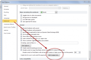
Edit Custom Lists in Excel

Edit Custom Lists in Excel

Custom Lists in Excel are great because the help to ensure accuracy and consistency when entering data on a worksheet. Excel comes with several Custom Lists built-in to the program – e.g. Days of the Week and Months of the Year. Now, you can quickly use Excel’s AutoFill handle to add Jan, Feb, Mar, Apr, etc. in any direction (vertical or horizontal) on the active worksheet.

Edit Custom Lists

You can quickly create – or edit – your own Custom List. Follow these steps:

  1. Type your list in a contiguous group of cells – either vertically or horizontally.
  2. Select the cells with the values that you just entered.
  3. Spell check this list – use the F7 Keyboard Shortcut
  4. Open up the Edit Custom List Dialog Box. (Watch this video to see how this is differs between Excel 2010, Excel 2007 and Excel 2003.)
  5. With your new Custom List selected, click the “Import” button to add your Custom List to the current version of Excel on this computer.

Sort Data Using a Custom List

On this video tutorial, I demonstrate how to sort a list of data using a Custom List – e.g. to get the “Month” field sorted in chronological order (January, February, etc.) This will save you a great deal of time!

Create a Custom List for Letters of Alphabet

Having a Custom List for the 26 letters of the alphabet comes in handy on many occasions. I show you how to AutoFill down the initial list using =Char(Row() + 64) beginning in Row 1 – a really usefuly function!

View This Excel Video Tutorial in High Definition

Follow this link to watch this video tutorial in High Definition on my YouTube Channel – DannyRocksExcels

Get my best-selling DVD-ROM, “The 50 Best Tips for Excel 2007” for only $29.97!

Share and Enjoy:
  • Add to favorites
  • Facebook
  • Twitter
  • Technorati
  • Print
  • email
  • Digg
  • StumbleUpon
  • del.icio.us
  • Yahoo! Buzz
  • Google Bookmarks
  • Orkut
  • SphereIt
  • Sphinn

How a Single Blank Cell Affects an Excel Pivot Table Report

As you will see in this Excel Video Tutorial, having a single blank cell in a data set will greatly affect how Excel Functions and Pivot Tables are designed and calculated.

Single Blank Cell in Data

Single Blank Cell in Data

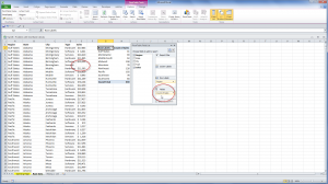
Imagine, how a single blank cell, in a field of 848 records, can change the way your Pivot Table views the data type (text vs. the expected numeric data type) and subtotal function (Count vs. the expected SUM function).

Seeing is believing!

Preventing a Blank Cell from “Creeping into” your data set

Use the Keyboard Shortcut Ctrl + Down Directional Arrow to go to the last cell that contains data in a column. This is a great way to isolate “stray” blank cells that will have a great impact on your Pivot Tables and other calculations in Excel.

Also, in Excel 2007 and Excel 2010, look for where a “numeric” field is placed by default. A single blank cell will cause an (intended) numeric field to be placed in the Row (text) labels area. Even dragging this field into the VALUES Drop zone does not solve the problem because the COUNT Function will be used to Subtotal this field. This is a “disaster waiting to happen!”

Introducing My Extended Length Excel Video Recordings

This is my opportunity to introduce you to my new, extended-length (one-hour +) Excel Video Tutorials that you can download for only US $9.95!

Here is the link that gives you more information about this exciting new service:

http://www.thecompanyrocks.com/pivot-table-tutorial-videos-to-download-practice-files-instructional-manual-included/

I offer you multiple options:

Let me know what you think!

Let me know which topics you would like me to record for you to download.

Send me an email with your comments and suggestions: danny@thecompanyrocks.com

Watch This Video in High Definition

Follow this link to view this Excel Tutorial in High Definition on my YouTube Channel – DannyRocksExcels

Share and Enjoy:
  • Add to favorites
  • Facebook
  • Twitter
  • Technorati
  • Print
  • email
  • Digg
  • StumbleUpon
  • del.icio.us
  • Yahoo! Buzz
  • Google Bookmarks
  • Orkut
  • SphereIt
  • Sphinn

Create a Custom Excel Function to Replace Formulas with Multiple IF Functions

Multiple Nested IF Functions

Multiple Nested IF Functions

Do you get tied up in a knot trying to write – let alone explain – a formula that has one IF Function nested inside another, and another…? I know that I do! And, what happens when your sales manager wants to revise the tiers for the quantity discounts? How many hours will this take you to review your logic and to make all of those multiple changes?

Usually, this will mean a lot of time, a lot of frustration and possibly some resentment thrown in as well!

Well, relax. I am going to demonstrate how easy it is to write a custom function in Excel using the “Select Case” Construct to replace the “rat’s nest” of multiple IF Functions in your formulas!

Scenario for this Function

You have been asked by your Sales Manager to write a formula to grant a discount, based upon the quantity of units ordered. There are 5 Tiers: Below 5 units ordered, no discount. From 6 to 24 units, a 10% discount, etc. Rather than spending a half hour nesting IF() functions and using AND() functions to create this formula, spend less than 10 minutes creating a Custom Excel Function instead.

Create the Custom Excel Function

  • Begin by opening the Visual Basic Editor. One way to do this is right-click any worksheet tab and select “View Code.”
  • Ensure that you have inserted a Module in the Project Explorer and that you have selected the module.
  • In the example that I use on this video tutorial, my first line of code is: “Function DiscQty(quantity)” and this is matched to an “End Function” statement
  • For this Custom Function, I am using the “Select Case” Construct in Visual Basic (VBA). Think of the keyword “Case” as a substitute for the =IF() Function.
  •  Rather than nesting the Excel =AND() Function inside the IF() Function, you will substitute – e.g. “Case 6 To 24” and then “DiscQty = 0.1” to indicate a 10% discount for quantities between 6 AND 24.

Watch the video to see how easy is is to create – and use – this custom Excel function. Invest the 7 minutes and 47 seconds to watch it – I guarantee that this investment of time will pay you many dividends for years and years to come!

View This Video Tutorial in High Definition

Follow this link to watch this Excel Video Tutorial in High Definition on my YouTube Channel – DannyRocksExcels.

Share and Enjoy:
  • Add to favorites
  • Facebook
  • Twitter
  • Technorati
  • Print
  • email
  • Digg
  • StumbleUpon
  • del.icio.us
  • Yahoo! Buzz
  • Google Bookmarks
  • Orkut
  • SphereIt
  • Sphinn

Write a Custom Excel Function to Link Worksheet Tab Name to a Cell

Custom Functions in Excel

Custom Excel Functions

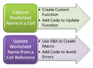
In response to many viewer requests, I am creating a two-part series of video tutorials that show you how to create links between the name of an Excel Worksheet Tab and a cell on that worksheet.

Here, in Part One, I demonstrate how to write a Custom Excel Function to capture the name of the worksheet tab in a cell.

Write Custom Excel Functions

You write Custom Excel Functions in the Visual Basic Editor. One way to open the Visual Basic Editor is to use the keyboard shortcut Alt + F11. Here are the elements that I use in this lesson:

  • Open the Project Explorer Pane (Keyboard Shortcut Ctrl + R).
  • Insert a Module to contain the VBA Code that you write for your Custom Function
  • Open the Code Pane (Keyboard Shortcut F7).

Write the Code for the Custom Function

In its simplest form, this is all of the code that you need for this Custom Excel Function:

Function SHEETNAME2() As String
SHEETNAME2 = Application.Caller. Parent.Name
End Function


That’s it!

Automatically Update Results of Custom Functions

A major difference between Custom Functions that you write and Excel’s Built-in Functions is that by default, the result of a Custom Function does not automatically update when values or references change. If you want your Custom Function to automatically update whenever the worksheet changes, add this line of code to your Custom Function in the Module:

Application.Volatile True

Source for this Code

I found the code for this Custom Excel Function in John Walkenbach’s Book, “Excel 2007 Formulas. He is an Excel Expert and I admire his writing style. You can check out his reources at this site:

http://spreadsheetpage.com/

Watch this Video in High Definition on YouTube

Click on this link to view this Excel Tutorial on my YouTube Channel – DannyRocksExcels.

Watch Part 2 of This Series

Here is the link to Part 2 in this Series. In this lesson I show you how to write an Excel Macro in VBA to update the Name of the Worksheet Tab based upon the value in a cell on the worksheet.

Share and Enjoy:
  • Add to favorites
  • Facebook
  • Twitter
  • Technorati
  • Print
  • email
  • Digg
  • StumbleUpon
  • del.icio.us
  • Yahoo! Buzz
  • Google Bookmarks
  • Orkut
  • SphereIt
  • Sphinn

How to Maintain Accurate Subtotals When Your Data Set Expands in Size

Subtotal in Excel 2010 Table

Subtotal in Excel 2010 Table

This is Part 2 of my series of video tutorials demonstrating how to use the SUBTOTAL Function in Excel.

  • In Part 1, I showed you the value of using the Subtotal Function to summarize the results of applying a Data Filter to a range of cells.
  • In this part, I show you how to use an Excel 2007 or Excel 2010 Table to ensure that your Subtotal Formulas are automatically updated when you append records or add additional fields to your original data set.

I strongly recommend basing Filtered Lists and Pivot Tables on an Excel Table (in Excel 2007 or 2010) or an Excel List in Excel 2003. This way, any formulas, filters and references that you make will be automatically updated when you append additional records or otherwise change the structure of your data set.

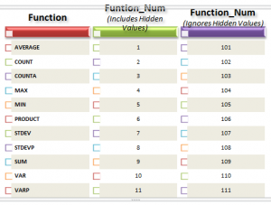
Function Numbers 101 through 111

Notice that when you “toggle on” the Total Row for a Table or List that Excel uses this formula = SUBTOTAL(109, Table1, [Sales]). Function 109 will use the SUM Function(109) to total the values in the “Sales” field ([Sales]) of a Table named “Table1.” These Function Numbers + 100 were introduced in Excel 2003 and the are automatically applied whenever you are using a Total Row in an Excel Table.

I think that you will learn some cool tricks in this lesson. Let me know what you think!

Watch This Video in High Definition

Click on this link to watch this video tutorial in High Definition, Full Screen Mode on my YouTube Channel – DannyRocksExcels.

Invitation to Visit My New Online Shopping Site

I invite you to visit my new, secure online shopping website – http://shop.thecompanyrocks.com

Once there, you can get my best-selling DVD-ROM, “The 50 Best Tips for Excel 2007”

Share and Enjoy:
  • Add to favorites
  • Facebook
  • Twitter
  • Technorati
  • Print
  • email
  • Digg
  • StumbleUpon
  • del.icio.us
  • Yahoo! Buzz
  • Google Bookmarks
  • Orkut
  • SphereIt
  • Sphinn

Don’t Subtotal Excel Data, Use Subtotal Function Instead

Subtotal Function

Subtotal Function Numbers

I used to love creating Subtotaled Reports. They are useful. They are easy to create. But they are also “clunky.” In my opinion, there are too many steps to take when you wish to see a Subtotal for a different field or to use a different function in your Subtotals.

Let me introduce you to the Subtotal Function in Excel. Here are several ways to take advantage of this function:

  • You can place the Subtotal Function in any cell on your worksheet – it does not have to reside directly below your data field.
  • You can use the Subtotal Function in connection with Data Filters – to get the subtotal for the visible cells in a filter.
  • You can use any of the 11 functions available to the Subtotal Function (Sum, Average, Count, etc.)

Watch This Video in High Definition on YouTube

This file size for this video is a little bigger than usual. So, to watch it, click on this link to view it in High Definition Mode on YouTube.

Subtotal Function Part Two

I have decided to film a second video lesson on the topic of the Subtotal Function – Using Subtotal Function in Excel Tables and Lists. Click on this link to watch my second video on this topic.

Watch or Download My 24 minute Introduction to Pivot Tables Video Recording

I have started to posted a series of “extended length” video tutorials online at: http://thecompanyrocks.webex.com – Follow this link to get more information about viewing or downloading my “free” Introduction to Pivot Tables.”

Get my best-selling DVD-ROM, “The 50 Best Tips for Excel 2007” for only $29.97!

Share and Enjoy:
  • Add to favorites
  • Facebook
  • Twitter
  • Technorati
  • Print
  • email
  • Digg
  • StumbleUpon
  • del.icio.us
  • Yahoo! Buzz
  • Google Bookmarks
  • Orkut
  • SphereIt
  • Sphinn

Two Ways to Turn Excel Data On Its Side – Transpose the Data!

Transpose Excel Data

Transpose Excel Data

How many times have you spent an hour or more creating an Excel worksheet only to discover – or be told – that you have the wrong structure? The values that you entered run vertically down in Column A. And  now, you need to have your values run horizontally across in Row 1.

Well, don’t despair! And, most important, do NOT retype your entries on another worksheet. Rather,watch this video to see how to “Turn Excel Data On Its Side”:

  1. Select Transpose from the Paste Select dialog box or the right-click shortcut menu
  2. Use the =TRANSPOSE() Function which is an Array Function

Watch as I demonstrate the advantages of each approach – they are different! If you are “curious” about how an Array Function works, the TRANSPOSE Function is a good one to practice with.

Click this link to watch this video in High Definition on YouTube.

Now Using Excel 2010

I filmed this video using Excel 2010. I will use Excel 2010 for all future video lessons unless there is a particular need to use another version to illustrate a point.

Download Workbook Used in This Video

Click on this link to download the Excel Workbook that I used in this video tutorial. It is stored on my “SkyDrive” at www.office.live.com

Get my best-selling DVD-ROM, “The 50 Best Tips for Excel 2007” for only $29.97!

Share and Enjoy:
  • Add to favorites
  • Facebook
  • Twitter
  • Technorati
  • Print
  • email
  • Digg
  • StumbleUpon
  • del.icio.us
  • Yahoo! Buzz
  • Google Bookmarks
  • Orkut
  • SphereIt
  • Sphinn

Create an Accounts Payable Summary Report in Excel

Accounts Payable Status Summary

Accounts Payable

Here is another video lesson that I created to answer a question from one of my viewers. In this case, the request is for help in creating an Accounts Payable Summary Report in Excel.

Formula to Create Label for Status

My viewer wants to know how to create one formula that will report the status of an Invoice as “Paid,” “Pay Now,” or “Delay.” To do this I “nested” one IF() formula inside another IF() formula. I used the ISBLANK() function as my first “logical test” in the formula. ISBLANK returns either TRUE or FALSE, so it is a good Function to become familiar with.

One of my “best practices” when learning how to “nest” IF Formulas, is to create each one separately – to test the results – and then copy and paste them into the combined formula.

Use SUMIF() Function to Total Status

Now, that your formula returns a status label for each invoice, you can use the SUMIF Function to search in the Named Range “Status” for the cells that match the criteria (Paid, Pay Now, Delay) and then Sum the Invoice Amounts for each category.

Watch This Video in High Definition on YouTube

Here is the link to my YouTube Channel, DannyRocksExcels, where you can watch this in High Definition.

Download this Excel Workbook

Follow this link to go to my Public SkyDrive to download this workbook to practice with.

Share and Enjoy:
  • Add to favorites
  • Facebook
  • Twitter
  • Technorati
  • Print
  • email
  • Digg
  • StumbleUpon
  • del.icio.us
  • Yahoo! Buzz
  • Google Bookmarks
  • Orkut
  • SphereIt
  • Sphinn

Dynamically Update a Cell with an Excel Worksheet Name

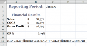
Formula to Capture Worksheet Name

Capture Tab Name in Cell

I am excited to share this Excel Tip with you! Several viewers have recently asked if there was a way to create a link in a cell to the name of a worksheet tab. Yes there is! And, in this lesson, I demonstrate how to do this.

Say, for example, that you want Cell C1 to contain the name of the current worksheet (Sheet1). With this formula, when you change the name of the worksheet to “January,” cell C1 is dynamically updated to show “January.”

Perfect for Excel Templates

If you use a template for your monthly, regional sales or financial reports, then this Excel formula is essential. You write the formula once – using Group edit – and each worksheet in your Excel workbook will be linked to a cell in your report. Change the name of the worksheet and your report name is automatically updated.

Functions Used in this Formula

  • CELL() – to gather information about the worksheet – in this case, the “Filename.”
  • MID() – to extract the characters in a text string – e,g, the “worksheet name.”
  • FIND() – to locate the starting point for the MID() function to extract the characters in the text.

As the final argument for the MID() Function, I use 31 characters because that is the maximum number of characters that you can use when naming an Excel worksheet.

Try this for yourself. Let me know how it works for you. Add your comments below.

Download Excel Workbook for this Lesson

Watch Video in High Definition

Follow this link to view this video tutorial on my YouTube Channel – DannyRocksExcels

I invite you to watch or to subscribe to my video podcast on iTunes. Follow this link to learn more about my RSS Feed.

Share and Enjoy:
  • Add to favorites
  • Facebook
  • Twitter
  • Technorati
  • Print
  • email
  • Digg
  • StumbleUpon
  • del.icio.us
  • Yahoo! Buzz
  • Google Bookmarks
  • Orkut
  • SphereIt
  • Sphinn