How to Place Dates in a Fiscal Year Quarter

Many organizations operate in a Fiscal Year – for example, April 1 through March 31 of the next calendar year. I get many requests from viewers for help with placing calendar dates into the proper Quarter for their Fiscal Year.

Excel Functions Used in Video TutorialWhile researching a question from one viewer, I cam across a very interesting formula that nests the “undocumented” DATEDIF() Function inside the CEILING() Function. I found this formula in the book, “Formulas and Functions with MS Excel 2003,” written by Paul McFedries. It is a very efficient formula.

What is Covered on the Video

Watch this video tutorial as I break down each step. As a Best Practice, I recommend that you break down a complex formula by working from the “inside out.” I start with the “nested” DATEDIF() function and then demonstrate the results of each formula detail.

Learn More About the “Undocumented” DATEDIF() Function

For various reasons, Microsoft does not offer any help or documentation for the very useful DATEDIF() Function. In fact, it is not even listed as a Function! However, it is very useful and often found in VBA (Visual Basic for Applications) coding. Here, are links to two videos that I created to help you understand how to use DATEDIF():

Learn How to Calculate a Calendar Year Quarter

In response to viewer requests, I created a companion video tutorial -” How to Calculate a Calendar Year Quarter in Excel.”

Resources Available at The Company Rocks

I invite you to visit my secure online shopping website – http://shop.thecompanyrocks.com – to preview the many resources that I offer for helping you to improve your software skills.

Watch Video Tutorial in High Definition

If you would like to watch my video tutorial for “Finding the Fiscal Year Quarter for any Date,” click on this link. I have posted it on my YouTube Channel – DannyRocksExcels

Watch this Video Now


Share and Enjoy:
  • Add to favorites
  • Facebook
  • Twitter
  • Technorati
  • Print
  • email
  • Digg
  • StumbleUpon
  • del.icio.us
  • Yahoo! Buzz
  • Google Bookmarks
  • Orkut
  • SphereIt
  • Sphinn

3 Reasons to Create and Use Named Ranges in Excel Formulas

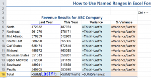
Use Named Ranges in Formulas

Use Named Ranges in Formulas

In my opinion, there are three reasons to use Named Range references in Excel Formulas:

  1. They are easier to write. Particularly, if you are referencing cells in another worksheet.
  2. They are easier to remember. Using =Sales – Cost of Goods Sold to determine Gross Profit vs. =A1 – B1
  3. They are easier to explain. Especially, if you are sending an Excel Workbook to a client or a colleague.

Creating Named Ranges in Excel

In this tutorial, I demonstrate two methods for creating a named range:

  1. Select the cells in the range and then type the name in the “Name Box” in the Upper Left Corner of the worksheet.
  2. Select both the cell with the “Name” and the adjacent cells for the range. Then use the Keyboard Shortcut Ctrl + Shit + F3 to open the Create Names from Selection Dialog Box

Remember that all Named Ranges MUST begin with a Letter or an Underscore and they CANNOT contain any Spaces!

Paste Named Ranges into Formulas

If you are using Excel 2007 or Excel 2010, you can take advantage of Formula AutoComplete to quickly and accurately include named ranges in your formulas. In ALL versions of Excel you can use the F3 Keyboard Shortcut to open the Paste Names Dialog Box and select the named range that you wish to paste into your formula.

Additional Resources for Excel

I invite you to visit my secure online shopping website – http://shop.thecompanyrocks.com – where you can preview all of the resources that I offer you.

Watch Tutorial in High Definition

Follow this link to watch my Excel Video in High Definition. My YouTube Channel – DannyRocksExcels – has received over 1 million views!

Watch Video Now

Share and Enjoy:
  • Add to favorites
  • Facebook
  • Twitter
  • Technorati
  • Print
  • email
  • Digg
  • StumbleUpon
  • del.icio.us
  • Yahoo! Buzz
  • Google Bookmarks
  • Orkut
  • SphereIt
  • Sphinn

How to Use Excel Formulas and Functions to Analyze Inventory for a Retail Store

Excel Formulas to Analyze Inventory

Excel Formulas to Analyze Inventory

My friend, Alan Friedman, is a CPA and Partner in Friedman Kannenberg and Company, PC. I have been using one of the Excel Worksheets that Alan developed to teach retail store owners and managers how to analyze their inventory. In this lesson, I demonstrate how to write and copy the Excel formulas needed to perform this analysis.

Excel Formulas for Analyzing Inventory

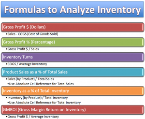
Many retailers use a Point-of-Sale (POS) System that can generate three numbers: Sales by Product Category, Cost of Goods Sold (COGS) by Product Category and Average Inventory by Product Category. Taking these three numbers – also known as “hard-coded” values – you can use Excel Formulas to give you:

  • Gross Profit Dollars (Sales minus COGS)
  • Gross Profit Percentage (Gross Profit Dollars divided by Sales)
  • Inventory Turns (COGS divided by Average Inventory)
  • Product Category Sales as a Percentage of Total Sales (Category Sales divided by Total Sales) – Use an Absolute Cell Reference
  • Inventory by Category as a Percentage of Total Inventory – (Inventory by Category divided by Total Inventory) – Use an Absolute Cell Reference
  • Gross Margin Return on Inventory (GMROI) – (Gross Profit Dollars divided by Average Inventory)

Tips for Entering and Copying Excel Formulas

As I demonstrate in this tutorial, you can write and copy an Excel Formula in one step when you first select the cells to receive the formula and use the Ctrl + Enter Keyboard Shortcut to complete the formula. Instead of clicking on the AutoSum Command or writing =SUM(), use the Alt + = (equal sign) to sum up the values in the adjacent range of cells.

Learn to Improve Your Excel Skills

If you want to learn how to create and use more Excel Formulas and Functions, I have created the Best-selling DVD-ROM, “The 50 Best Tips for Excel 2007.” You can learn more about this resource by visiting my secure online shopping website – http://shop.thecompanyrocks.com

Watch Tutorial in High Definition

I produce my Excel Tutorials in High Definition. Follow this link to view this lesson on my YouTube Channel – DannyRocksExcels

View Tutorial Now

Share and Enjoy:
  • Add to favorites
  • Facebook
  • Twitter
  • Technorati
  • Print
  • email
  • Digg
  • StumbleUpon
  • del.icio.us
  • Yahoo! Buzz
  • Google Bookmarks
  • Orkut
  • SphereIt
  • Sphinn

The Basics for Creating and Copying Formulas and Functions in Excel

Relative and Absolute Cell References

Relative and Absolute Cell References

Formulas and Functions are the “core elements” of Excel. It is vital that you have a solid grounding in understanding how formulas and functions work; especially when you need to copy and paste them into other cells.

Relative and Absolute Cell References

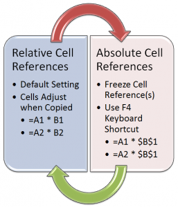
When you use Relative Cell References – the default setting in Excel – the Row numbers and Column letters adjust automatically when you copy and paste a formula.

There are, however, situations where you need to “freeze in place” part of an Excel Formula. For example, you need to “freeze” or use an Absolute Cell Reference to the cell with “Total Sales,” when creating and copying a formula to determine Product Sales as a Percentage of Total Sales.

Copying Excel Formulas

In this tutorial, I demonstrate two methods for copying and pasting formulas and functions:

  • Standard Practice is to select the cell with the formula and use the Ctrl + C Keyboard Shortcut to place the formula cell on the Excel clipboard. Then, after selecting the destination cell(s), use the Ctrl + V Keyboard Shortcut to paste the formula in the new location(s)
  • AutoFill Tool.If you are copying the formula cell into adjacent cells, use the AutoFill tool to do this quickly and accurately!

Tips that You May Not Know

In my experience, many Excel veterans are not familiar with these tips and tricks which I demonstrate in this tutorial:

  • The Ctrl + ~ (tilde) Keyboard Shortcut to “toggle” the Show Formulas view for the active Excel Worksheet.
  • The Alt + Enter Keyboard Shortcut to automatically use the =SUM() Function – for adjacent cells.
  • The F4 Key to automatically add Absolute Cell Reference when creating or editing a formula. For example, converts A1 to $A$1.

Learn More Excel Tips and Tricks

50 Best Tips for Excel 2007

50 Best Tips DVD-ROM

If you enjoy the tips and techniques that I demonstrate in this lesson, then you will really benefit from purchasing my best-selling DVD-ROM, “The 50 Best Tips for Excel 2007.” You can learn more about the resources that I offer by visiting my secure online shopping website – http://shop.thecompanyrocks.com

Watch Tutorial in High Definition

Follow this link to view this Excel tutorial in High Definition on my YouTube Channel – DannyRocksExcels

Play Video Now

Share and Enjoy:
  • Add to favorites
  • Facebook
  • Twitter
  • Technorati
  • Print
  • email
  • Digg
  • StumbleUpon
  • del.icio.us
  • Yahoo! Buzz
  • Google Bookmarks
  • Orkut
  • SphereIt
  • Sphinn

How to SUM Values in One Field Based on Criteria from Multiple Fields in Excel

SUMIFS and DSUM Functions

SUMIFS and DSUM Functions

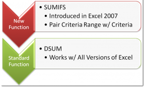
The new SUMIFS() Function was introduced in Excel 2007. With SUMIFS, you can sum the values in one field based up criteria that comes from multiple fields. This is a very valuable Function.

SUMIFS Function

The key to understanding SUMIFS, is that you “pair” a criteria range with the criteria for that range. As you watch my tutorial, the importance of this concept will become clear to you.

DSUM Function

If you are using – or need to create workbooks that are compatible with – older versions of Excel – e.g. Excel 2003, you can use the DSUM Function to achieve the same results. The DSUM belongs to the Database Functions set in Excel.

Use Named Cell Ranges in Formulas

I highly recommend that you learn how to create – and then use – named cell references in your Excel Formulas and Functions. In this tutorial, I show you how to do this. Once you have created a named cell reference, you can use the F3 Keyboard Shortcut to show a dialog box that lists all of the named Ranges that you can post into your formulas. This will save you time and help to ensure accuracy in your formulas – especially when you cop a formula to another location.

Bonus: Create Drop-down Menu with Data Validation

When using Multiple Criteria, I like to be able to select my criteria values from a drop-down list. In this lesson, I demonstrate how to do this using Data Validation in Excel.

Learn More Excel Tips

I invite you to visit my new, secure, online shopping website – http://shop.thecompanyrocks.com. Here, you can learn more about the tips on my best-selling DVD-ROM, “The 50 Best Tips for Excel 2007.”


Watch Video in High Definition

Here is the link to view this Excel Tutorial in High Definition on my YouTube Channel – DannyRocksExcels

YouTube Video

Share and Enjoy:
  • Add to favorites
  • Facebook
  • Twitter
  • Technorati
  • Print
  • email
  • Digg
  • StumbleUpon
  • del.icio.us
  • Yahoo! Buzz
  • Google Bookmarks
  • Orkut
  • SphereIt
  • Sphinn

How to AutoFill the Letters in the Alphabet in Excel

 One of my viewers would like to be able to AutoFill the Letters in the Alphabet in his Excel Workbooks – he creates Alpha-Numeric Part Numbers for his products.

Two Ways to AutoFill Letters in the Alphabet

  1. Use a Formula – =CHAR(ROW(A65)) and AutoFill Down in the Column – This is not ideal
  2. Create and Use a Custom List in Excel. – So, use the Formula to create your list of 26 Alphabetical Letters. Copy the List and use Paste Special Values to convert the formulas to values. Then create your Custom List.

Using the CHAR() Function in Excel

There are 255 ASCI Characters that you can use in Formulas. For example, =CHAR(169) will return the © Symbol. In this lesson, I share a great Keyboard Shortcut that you can use to add this Symbol into the Footer of your printed Excel worksheet – Watch the video to discover this!

Visit My Secure Online Shopping Site

I hope that you take a few minutes to visit my new, secure online shopping website. The address is: http://shop.thecompanyrocks.com


Watch Tutorial in High Definition

On my YouTube Channel – DannyRocksExcels – I have posted this tutorial in High Definition Mode. Click here to go directly to this video.


Share and Enjoy:
  • Add to favorites
  • Facebook
  • Twitter
  • Technorati
  • Print
  • email
  • Digg
  • StumbleUpon
  • del.icio.us
  • Yahoo! Buzz
  • Google Bookmarks
  • Orkut
  • SphereIt
  • Sphinn

Tips for Working with Array Formulas and Functions in Excel

Using ARRAY Functions in Excel

ARRAY Formulas in Excel

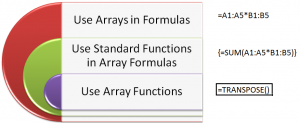
Array Formulas and Functions are very powerful tools to use in Excel. However, the concept of working with ARRAYs take a little bit of time and practice. In this video tutorial, I demonstrate how to:

  1. Create formulas that use ARRAYS as arguments
  2. Work with ARRAY FUNCTIONS – for example, the TRANSPOSE Function
  3. Key “Got’cha” steps to master – for example, selecting all cells to receive formula results before creating the ARRAY Formula.
  4. The importance of using Ctrl+Shift+Enter to complete the Array formula.

What is an ARRAY?

“An Array is a collection of Cells or Values that Excel treats as a single unit.”

Why Use an ARRAY Formula?

  1. Automatic Level of Protection for Formula Cells – You cannot delete nor edit a single cell in an Array Formula
  2. Eliminate Intermediary Calculations – For example, you can find the Grand Total without having to create a field to calculate “Extended Price.”
  3. Worksheet, usually, calculates faster because you are using fewer formulas.

Visit My NEW Online Shopping Website

http://shop.thecompanyrocks.com is my new, secure online shopping website. I invite you to visit and preview my new products.

Watch Tutorial in High Definition

Follow this link to view this tutorial in High Definition on my YouTube Channel – DannyRocksExcels

Share and Enjoy:
  • Add to favorites
  • Facebook
  • Twitter
  • Technorati
  • Print
  • email
  • Digg
  • StumbleUpon
  • del.icio.us
  • Yahoo! Buzz
  • Google Bookmarks
  • Orkut
  • SphereIt
  • Sphinn

How to Use the Solver Add-in for Excel – Part 2

Solver Parameters

Solver Parameters

This is Part 2 of my series of video tutorials where I demonstrate how to use the SOLVER Add-in Tool in Excel to produce a specific result for a formula.  Remember that SOLVER is an Add-in program that you must activate before you can use it. Watch Part 1 in this series to learn how to activate SOLVER.

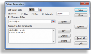
In this tutorial, I work with the same data set that I used in Part 1. This time, I want to achieve a specific amount of Gross Profit Sales Dollars. First, however, I must determine what is a reasonable amount to set as the Target for Solver to return.

Use SUMPRODUCT Function in Excel

I use the SUMPRODUCT Function to quickly determine my possible Revenue, Cost of Goods Sold and Gross Profit is I sell all of the Units that I have in stock. Now, I have a reasonable Target for SOLVER to reach. SUMPRODUCT is a very efficient Function that, unfortunately, very feel Excel users – in my experience – know about. Follow this link to my Index of Excel Video Lessons to find additional tutorials for SUMPRODUCT.

Best Practice Tips for Solver

  • Work with a copy of your worksheet. This is always a good idea, and it is most important when you are beginning to learn how to work with SOLVER.
  • Write out your Goal for SOLVER.
  • Do you want SOLVER to Maximize the Formula? For example, to Maximize your potential profit?
  • Do you want SOLVER to Minimize the Formula? For example, to Minimize your costs?
  • Do you want SOLVER to return a Specific Number? If so, what is that number?
  • Determine your “Variable Cells.” SOLVER calls them the “By Changing Cells.” These are the cells that SOLVER will automatically adjust.
  • The Variable Cells must “feed int” the formula in your Target Cell – This is the key to making SOLVER work!
  • Write out your “Constraints.” These are the “real-world” conditions that you want SOLVER to operate under. This is the real power in SOLVER.
  • Do not treat the SOLVER results as “the Gospel.” SOLVER is a powerful Business Intelligence Tool. You, however, know your own business or industry. Use SOLVER as a tool to help you to make informed business decisions.


Watch Part 1 in SOLVER Series of Video Tutorials

Watch Tutorial in High Definition

Follow this link to view this Excel Tutorial in High Definition on my YouTube Channel – DannyRocksExcels.

Share and Enjoy:
  • Add to favorites
  • Facebook
  • Twitter
  • Technorati
  • Print
  • email
  • Digg
  • StumbleUpon
  • del.icio.us
  • Yahoo! Buzz
  • Google Bookmarks
  • Orkut
  • SphereIt
  • Sphinn

How to Create a Summary Report from an Excel Table

Functions for Executive Summary

Functions for Executive Summary

I created this Excel Video Tutorial in response to a viewer who, in her company, is not permitted to use a Pivot Table to create a report. Unfortunately, this happens more often than you might think. Nevertheless, I promised to share my tips and advice. I think that many of this tips will help Excel users at all levels.

Tips Covered in this Video Tutorial

  • Use Advanced Filter to Extract a list of unique customer names from a range with @ 4,300 records.
  • Later in the lesson, I show you how to extract this list to a different worksheet – a tip that will save you time when preparing your reports!
  • How and why to convert a normal range of data into a TABLE in Excel 2007 / 2010 or into a LIST in Excel 2003.
  • How to create “Named Ranges” for your key data cells and to use them in your Formulas and Functions.
  • How to use the SUMIF, AVERAGEIF and COUNTIF Functions in your summary report.

Keyboard Shortcuts Used in this Tutorial

  • Ctrl + T to convert to a TABLE in Excel 2007 / Excel 2010
  • Ctrl + L to convert to a LIST in EXCEL 2003
  • Ctrl + A to open up the Function Arguments Dialog Box
  • Ctrl + Shift + F3 to open the Create Names Dialog Box
  • F3 to open the Paste Names Dialog Box

I decided that I will only make this video available on YouTube – I think that you will enjoy the clarity that you get from the High-Definition / Full Screen Mode.

Watch Tutorial in High Definition on YouTube

Follow this link to view this Excel Tutorial in High Definition on my YouTubeChannel – DannyRocksExcels

Visit my new secure online shopping website

I invite you to visit http://shop.thecompanyrocks.com – my new online shopping website.

Watch Video Now

Share and Enjoy:
  • Add to favorites
  • Facebook
  • Twitter
  • Technorati
  • Print
  • email
  • Digg
  • StumbleUpon
  • del.icio.us
  • Yahoo! Buzz
  • Google Bookmarks
  • Orkut
  • SphereIt
  • Sphinn

How to Use Criteria in Excel Functions and Filters

Criteria for Advanced Filter

Criteria for Advanced Filter

When you apply a Filter to an Excel data set, you use Criteria. In a filter, only the records that can answer “TRUE” to the criteria that you set will appear. The records that answer “FALSE” are hidden while the filter remains in place.

Logical Functions

The IF(), AND() and OR() Functions belong to a group of Logical Functions. In their function arguments, they evaluate a “Logical Test” and can perform one action is the answer is “TRUE” and a different action if “FALSE.” 

  • The AND() Function – each of the Logical Tests must be met in order to return the answer “TRUE.”
  • The OR() Function – if any condition is met, the answer that is returned is “TRUE.”
  • I frequently “Nest” an AND() Function or an OR() Function inside an IF() Function to test multiple criteria.

Advanced Filters in Excel

While many Excel users are familiar with Filtering, in my experience, I find that many people get confused when it comes to using Advanced Filters. In this video tutorial, I try to eliminate this confusion. Watch and you will learn how to:

  • Write Criteria for Advanced Filters using “AND” criteria and “OR” Criteria.
  • Copy the “Filtered Records” to another location
  • Use the Keyboard Shortcut Ctrl + Shift + L to quickly “toggle” normal filter drop-down menus on or off.


Watch Tutorial in High Definition

Follow this link to watch this Excel Tutorial in High Defintion on my YouTube Channel – DannyRocksExcels

Share and Enjoy:
  • Add to favorites
  • Facebook
  • Twitter
  • Technorati
  • Print
  • email
  • Digg
  • StumbleUpon
  • del.icio.us
  • Yahoo! Buzz
  • Google Bookmarks
  • Orkut
  • SphereIt
  • Sphinn