Creating Combination Charts in Excel

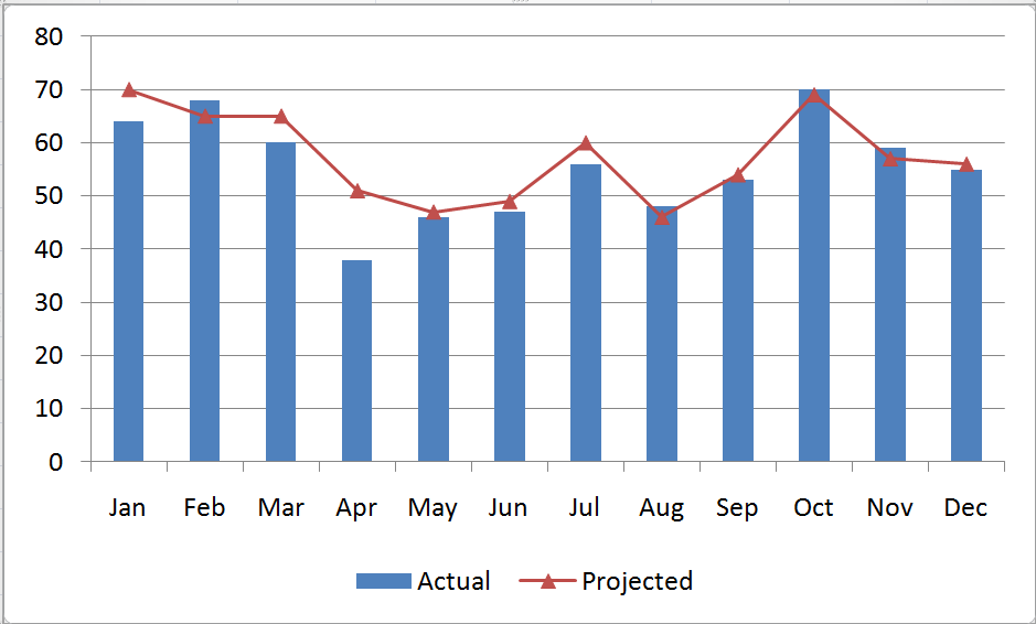
A combination chart in Excel is not a single chart type. Rather, you create combination charts by combining two or more complementary chart types. The most common combination is a Column type for one series and a Line type chart for the second series. Combination Charts, in general, make it easier to spot or highlight the trends in your data.

Combination Chart

Excel Combination Chart

 Creating a Combination Chart

  1. Create a standard chart for your data.
  2. Select one series and then choose a different chart type for that series.
  3. Make formatting choices as necessary.

Adding a Secondary Axis for Data

When you are comparing data series that have a wide “gap” between them – e.g. comparing actual sales in a month (large number) – to Profit % in each month (small number), you will want to create a Secondary Vertical (Value) Axis in your Combination Chart.

Begin by selecting the series that you want to plot and Right Mouse Click to Format the Series on a Secondary Vertical Axis. I recommend that you add in Axis Titles for both the Primary and Secondary Vertical Axes.

Formatting Charts in Excel 2007 and 2010

Charting in Excel – beginning with Version 2007 – now offers quite a few professional graphic design elements. In this video lesson, I show you how to customize the presentation of your graphical image. You can make these changes with just a few mouse clicks! It is definitely worthwhile to learn how to improve the visual impact that your Combination Charts make.

Learn how to “Master Excel in Minutes – Not Months!”

Follow this link to watch this Excel Video in High Definition, Full Screen Mode on my YouTube Channel – DannyRocksExcels

Subscribe to or watch my – free – video podcast on iTunes.
Click & Drag a Data Series to Goal Seek in Excel

Did you know that you can click on a Data Series in an Excel Chart and “drag it to reach a new value?” You can!

Changing the data value in your chart brings up the Goal Seek Dialog Box. Now, it is a simple matter to confirm your new value and tell Excel which cell reference to change in your formula. Instantly, your chart redraws and your data and formula are updated with the substitute value – and your NEW GOAL!

Here are the steps to follow in this Excel Video Lesson:

  1. I use the =FV() Function to show the future value of my investment for each year that we invest. The =FV() Function requires a “fixed” interest rate and a constant investment value contributed each period.
  2. I inserted a “Line” type chart onto my worksheet – i.e. I “embedded” the chart on the sheet.
  3. I used a “Custom Format” on the Value Axis for our numbers (#,##0,K) to show the numbers as thousands ($80K)
  4. For this chart, I also changed the “Maximum Value” of the Value Series by typing in a new (higher) number.
  5. To reach a “new goal” on our chart, first click to select the data series. Then click again and drag the data line to a new point on the chart.
  6. This brings up the “Goal Seek” Dialog Box. Edit your new goal if necessary. Then click on the cell that you want to change in order reach your goal. That cell must be referenced in your formula. The chart redraws and your formula results are updated.

Find the Excel Video Lesson that you want – Index of all Excel Topics

News! My DVD, “The 50 Best Tips for Excel 2007” is now available to purchase. I invite you to visit my online bookstore for more details.