Using the Built-in Excel Data Form to Edit, Enter and View Records

Data Form in Excel

Data Form

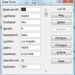
Excel has a built-in Data Form which is very useful for viewing all of the fields (up to 32 of them) associated with a single record. When you have lots of “Fields” in your “Data Set” and you do not want to do a lot of horizontal scrolling to view or edit the values in the cells, use this Data Form.

There is a limit of 32 fields when using Excel’s built-in Data Form.

Customize the Quick Access Toolbar

However, it does not appear as a Ribbon Command in Excel 2007. To use the Data Form add the Form Command to your Quick Access Toolbar (QAT) – I show you how to do this in the video.

Personally, I do not recommend the Excel Data Form for entering new records in your data set. I like to add Data Validation drop-down lists to ensure data integrity and this feature is not available in the Data Form. However, you can use Criteria to quickly find records for viewing and editing in the form.

Filtering Data with the Data Form

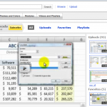
I give you a brief introduction to some of the new filtering options available in Excel 2007. I will cover this in greater detail in another lesson.

Subscribe to My Video Podcast on iTunes

I invite you to subscribe to my free video podcast, “Danny Rocks Tips and Timesavers” on iTunes. Click here to go directly to my iTunes podcast. I have had over 25,000 downloads since I began my podcast in June of 2010.

Watch this video in High Definition

Click here to go to my DannyRocksExcels YouTube Channel.

Watch Video Now

Master Excel in Minutes Video Training Resources

I have created a series of extended length Excel Video Training Resources. I invite you to visit my secure online shopping site to: Learn how to “Master Excel in Minutes – Not Months!”

My Most Viewed and Downloaded Videos for Excel and PowerPoint

My iTunes Podcast

Danny on iTunes

I began to post my videos as podcasts at the iTunes store this past summer. Since then, my video lessons for Excel and PowerPoint have been viewed and downloaded many times. I am thirlled. And, I thank you for your support and encouragement.

Here are the links – on my website – to the most popular video episodes. I have organized them by category in the order of their popularity. You can click on any link to view or download that video from my website. Or, you can go to my video Podcast by clicking on this link – “Danny Rocks Tips and Timesavers” Podcast on iTunes.

Merging and Consolidating Excel Worksheets

 PowerPoint Presentations

Data Visualizations

What-If Analysis in Excel

Importing Data From Other Programs

Pivot Tables

Excel Tables

Social Media

Formula Errors

Please add your comments below – or on my iTunes Channel. I welcome your feedback.

You can learn how to “Master Excel in Minutes – Not Months!”

Sincerely,

Danny Rocks

How to Annotate Excel Worksheets with Comments and Images

Do you use “post-it” sticky notes to remind you how to do something? Do you ever lose your reminder notes? I know that I do! So that is why I like to annotate my Excel Worksheets with Comments – this way I have the notes properly located (in the worksheet) when I need them (to remember how to write a particular formula, etc.) the most!

In this lesson, I also show you how to add “pictures” inside your comments. This is a great tip for adding in a picture for a catalog or order form.

A question that I am frequently asked: “How do I print out my comments?” Watch this video to find out how to do this – there are a couple of “got’cha” steps involved.

Logo for The 50 Best Tips

The 50 Best Tips

Here are three ways to enter a new comment that is attached to a single cell:

  • Use the Keyboard Shortcut Shift + F2
  • Right-Mouse Click and choose “Insert Comment”
  • On the Review Tab of the Ribbon (Excel 2007) select the “Insert New Comment” command.

You can edit your comments, re size the shape of your comments, hide your comments (only a “red triangle” shows in the cell until you hover near the cell), show your comments (individually or collectively), delete, clear and paste your comments. I cover each of these techniques in this video lesson. And more!

Watch this video in High Definition, Full Screen Mode on my YouTube Channel – DannyRocksExcels

Learn how to “Master Excel in Minutes – Not Months!”

How to Use the Indirect Function to Create Excel Dashboards

You can use the Indirect Function to create an Excel Dashboard. A Dashboard gives you an overview of your data – in this case, an interactive view of the information hidden in our data set. I will create Drop-Down lists using Data Validation in the Dashboard. The Indirect Function takes a little bit of time to understand. Here are some key points:

  • The Indirect Function works best with Named Cell References
  • The syntax is =INDIRECT(reference text). In our example the “reference text” will be the label for a Named Range of cells.
  • You can “nest” the Indirect Function inside another function – e.g. =SUM(INDIRECT())

Later in the lesson, I show you how you can quickly  look up any cell at the “intersection” of a Named Row and a Named Column – e.g. April East. You use the SPACE BAR as the “Intersection Operator” to point to the cell where “April” meets “East.”

50 Best Tips for Excel 2007

Excel Tips

Some of the Keyboard Shortcuts that I use in this lesson are:

  • Ctrl + A to select all of the cells in a Data Set
  • F3 to bring up a list of all the Named Ranges that have been created in the current workbook
  • Ctrl + Shift + F3 to create Named Ranges for the cells in the selection – using as Names, the Labels in the Top Row / Left Column

Here is a link to the 1st lesson in this series on the INDIRECT Function in Excel.

Follow this link to watch this lesson in High Definition, Full Screen Mode on YouTube.

You can learn how to “Master Excel in Minutes – Not Months!”

How to Trigger a Unique List of Values Based Upon Another Drop-Down List in Excel

You can use the INDIRECT() Function in Excel to create a drop-down list of unique values that is“triggered” by the label that you select in another drop-down list. In the scenario that I use in this lesson:

  1. Create your 1st Drop-down list using Data Validation in Excel – Allow “List.” Here the named range is “Departments.”
  2. Create a 2nd Drop-down list using Data Validation. This time the “list” uses the INDIRECT Function to reference the selected label from the 1st drop-down list.

Key Concept

 The labels in my 1st drop-down list serve as “named range” references. That is why the INDIRECT Function is able to pull up the correct list of “Job Titles” in the 2nd Drop-down list. For example, a reference to the text label “Sales” in the 1st drop-down list brings up a list of the values (Job Titles) from the “Named Range” (Sales) in the 2nd Drop-down list.

If you need to learn about – or review – Data Validation in Excel, follow this link to my free Excel video lesson on this topic.

Create Named Ranges in Excel

I have found that creating and using “Named Cell Range” references makes lookup functions and formulas so much easier in Excel. Watch this video to see how I use a variety of methods to Create Named Ranges in Excel. One tip is to use the Keyboard Shortcut “Ctrl + Shift + F3” – after you first select the Label and the Values for your Named Range.

In this lesson, I also demonstrate how to visually “flag” all of the cells that do not meet the criteria for your Data Validation. I find that most people are unaware that you can do this! I think that you will find many uses for this auditing tool as you work in Excel.

Additional Resources

Follow this link to watch this video on YouTube in High Definition, Full Screen Mode.

Here is the link to view the 2nd video in this series about the INDIRECT Function in Excel.

Learn how to “Master Excel in Minutes – Not Months!” – visit my new, secure shopping site – http://shop.thecompanyrocks.com

How to Add a Data Validation Drop Down List to an Excel Form

Several viewers wrote to me after I posted my previous video – “How to Add a Combo Box Control to an Excel Invoice Form” to suggest that there is another way to create a “drop down list” for a form. Yes, you can use Data Validation in Excel and use “Allow from List” as your setting. Use the “Stop Style” to prevent a user from typing in a value that is not in the list.

In this Excel Training Video I compare both approaches: Using a Combo Box Control and Adding a Data Validation Drop Down List. Both work well on Invoice Forms. However, you will use a different function to “lookup” other values – e.g. Unit Price – depending upon your choice:

  • With a Combo Box Control, use the =INDEX() function to find the “Unit Price” for the product selected in the Combo Box
  • With a Data Validation Drop Down List, use the =VLOOKUP() function to find the matching “Unit Price.”

Let me know which approach that you prefer. Try both – expand your Excel Skill Set. Add your comments below or send me an email with your thoughts and suggestions: danny@thecompanyrocks.com

You can start to shop for my DVD, “The 50 Best Tips for Excel 2007” by clicking this link.

Learn how you can “Master Excel in Minutes”

How to Use Excel Lookup Functions to Create a Customer Invoice

Excel has many powerful Lookup Functions. You can use them, for example,  to lookup an Item Number when you know the Product Description. Or to automatically look up the List Price for an Item Number on your customer invoice. In this lesson I show you how to use three Excel Lookup Functions:

  1. The INDEX() Function
  2. The MATCH() Function
  3. The VLOOKUP() Function

I hope that you enjoy learning – and applying – these techniques. I would like to hear from you, so you can either add a comment below or send me an email.

You can receive my new Tips and Timesavers Videos automatically by subscribing to my RSS Feed or to my free podcast on iTunes. Click here to view, download or subscribe to my podcast.

You can purchase any of my 5 DVDs in “The 50 Best Series …” for Excel 2007, PowerPoint 2007, Word 2007, Outlook 2007 and Access 2007 – Click here to open your shopping cart!

Learn how to “Master Excel in Minutes – Not Months!”

How to Use an Excel Data Table for “What-if” Analysis

Excel has many tools that give you answers to “What-if” questions. An Excel Data Table allows you to feed a series of “substitute values” into two arguments in a formula. For example, with a Data Table you can:

  • See a table of monthly payments on a loan by substituting both the “Interest Rate” and the “Amount Borrowed” simultaneously.
  • See a table of “Net Payments” by changing both the “Sales Price” and the “Quantity” simultaneously.
  • See the amount that you “tip” a service professional by changing both the “Tip Percentage” and the “Food Total” simultaneously.

As you will see in this Excel Video Lesson, the trick is to understand which series of values are the “Row Inputs” and which series of substitute values are the “Column Inputs.”

Trust me on this: It is easier to “see” how to set up a Data Table than it is to “write a description” of a Data Table. So, I invite you to “see for yourself” how easy it is to set up an Excel Data Table and get answers to two simultaneous “What-if” questions!

Click here to see a Listing of “The 50 Best Tips for Excel 2007.”

Learn how to “Master Excel in Minutes – Not Months!”

Prevent Duplicate Cell Entries with Excel Data Validation

Unfortunately, it is much too easy for a data entry clerk to assign duplicate account numbers. And this is a disaster waiting to happen. To prevent this from happening, use Excel’s Data Validation tool. In this short video lesson, I show you how to use the =COUNTIF() function in the Data Validation dialog box to ensure that only unique account numbers can be assigned to your customers.

I also show you how to extend the range of cells that contain this data validation rule: You use the Paste Special – Validation command.

This is one of “The 50 Best Tips for Excel 2007.” Click here to purchase the DVD using my secure shopping cart.

Learn how to “Master Excel in Minutes – Not Months!”

View My Excel Training Videos on YouTube

DannyRocksExcels on YouTube

YouTube

Two years ago, in August 2010, I started uploading my Excel video training lessons to my YouTube Channel – DannyRocksExcels. Now there are 93 Excel videos available. I was originally reluctant to post my video content on YouTube because I selfishly wanted to restrict my videos to my own website. After a conversation with a colleague, I changed my mind and began to upload all of my Excel videos to YouTube.
Why?
  • YouTube attracts a much more diverse audience than I could ever hope to attract on this website.
  • YouTube makes it easy to download and share my videos with others.
  • YouTube has a great analytics program – Insight – that allows me to gain valuable information about my audience.
  • YouTube is now showing several of my most popular videos as ads automatically (via Google AdSense)
  • I have good interaction with my viewers on YouTube – comments, requests for new videos, etc.

When I look at the numbers on YouTube I am amazed!

Here is a summary:

  • My Excel Videos have been viewed almost 200,000 times over the past two years.
  • One Video (Introduction to Pivot Tables) has been viewed over 20,000 times!
  • My DannyRocksExcels Channel on YouTube now has over 500 subscribers.

I invite you to view, download or subscribe to my YouTube Channel for Excel Training videos by following this link.

Thank you!

Danny Rocks

P.S. Learn how to “Master Excel in Minutes – Not Months!”