Use an Excel Template to Customize a Worksheet with 52 Weeks of Employee Time Cards

Template for Time Cards in Excel

Time Card Templates in Excel

This is Part Two in my new series of Excel Tutorials where I share my best practice tips for creating 52 weeks of Employee Time Cards – for hours worked. In this segment, I focus on starting the process with an Excel Template.

Finding Templates for Time Cards

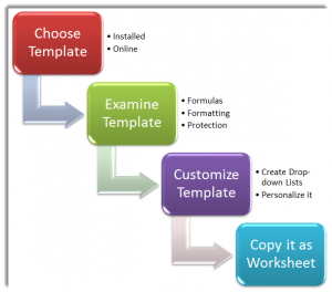
As I demonstrate in the video, there are at least two easy sources for finding a Time Card Template:

  1. Sample Templates Installed on your Computer
  2. Templates that you can preview and download from the Microsoft Office Templates Website

Examining Templates that You Download

Before you even think about duplicating the Excel Template that you just downloaded, it is important for you to take a few minutes to explore:

  • The Formulas used in the Template
  • The Formatting used in the Template – especially the formatting for Dates and Times
  • The Protection Applied (if any) to the cells or the entire worksheet

Creating Drop-down Menus for your Template

Since our premise here is that we will copy the template to 51 additional worksheets, it makes sense to use Data Validation to create a series of “drop-down menus” for Employee names and the Start Date for each week. I demonstrate how to do this in the video tutorial.

Links to Additional Video Tutorials in this Series

Additional Resources for Excel

I invite you to visit my new, secure, online shopping website – http://shop.thecompanyrocks.com – to discover the many training resources that I offer you!

Watch Tutorial in High Definition

Follow this link to watch this Excel Tutorial in High Definition on my YouTube Channel – DannyRocksExcels
Click to Watch Video Now

Share and Enjoy:
  • Add to favorites
  • Facebook
  • Twitter
  • Technorati
  • Print
  • email
  • Digg
  • StumbleUpon
  • del.icio.us
  • Yahoo! Buzz
  • Google Bookmarks
  • Orkut
  • SphereIt
  • Sphinn

Tips for Creating 52 Weeks of Employee Time Cards in Excel

Insert & Copy Worksheets

Insert & Copy Worksheets

We are now winding down the end of the year 2011. Several of my viewers and clients have asked my for help in creating one Excel Workbook that will contain 52 weeks of employee time card information:

  • Name and Department of Employee
  • Hours Worked each day of the week – Regular and Overtime
  • Number of Holiday / Sick Days that were used / that remain, etc.

First Tutorial in this Series

Rather than trying to create each individual – and some are very specific – request, I have decided to combine multiple requests into a series of Best Practice Tips for my general audience to consider.

In this lesson, I demonstrate:

  • Two methods for adding new blank worksheets to the Excel workbook
  • Two Methods for inserting an exact copy of an existing – and formatted – worksheet
  • My favorite tip – Fill Across Worksheets – either the formatting only, the contents only or the default setting – both formatting and contents.

Links to Additional Tutorials in this Series

Watch Tutorial In High Definition

Follow this link to watch this tutorial in High Definition on my YouTube Channel – DannyRocksExcels

Additional Resources at My Online Shopping Website

I invite you to visit my new – secure – online shopping website – http://shop.thecompanyrocks.com – and preview the many tutorials and resources that I offer you.

Watch Tutorial Now

Share and Enjoy:
  • Add to favorites
  • Facebook
  • Twitter
  • Technorati
  • Print
  • email
  • Digg
  • StumbleUpon
  • del.icio.us
  • Yahoo! Buzz
  • Google Bookmarks
  • Orkut
  • SphereIt
  • Sphinn

Excel Keyboard Shortcuts for Navigating Between Cells, Worksheets, Documents and Programs on your Computer

Excel Keyboard Shortcuts

Excel Keyboard Shortcuts

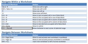
This is the latest installment in my series of Video Tutorials for Keyboard Shortcuts in Excel. This time the focus is on Keyboard Shortcuts for Navigating between:

  • Cells in a worksheet. For example, to move to the last “occupied” cell ( a cell with data) in a column or row
  • Worksheets in the active Workbook
  • Other Excel workbooks or documents that are open on your computer
  • Other programs that are open on your computer

Links to Other Videos in Keyboard Shortcuts Series

Here is the link that will take you to the other Video Tutorials that I have created for Excel Keyboard Shortcuts.

Download the Complete – FREE –  “Chart of Popular Keyboard Shortcuts for Excel.”

There are two ways for you to download – for FREE – My “Chart of Popular Keyboard Shortcuts for Excel:”

  1. Click here to download this – for FREE – at my new, secure online shopping website.
  2. Click here to download this – for FREE – from my Exclusive Membership Content page.

Watch Tutorial in High Definition on YouTube

Follow this link to view this Excel Tutorial in High Definition on my YouTube Channel – DannyRocksExcels

YouTube Tutorial for Excel Keyboard Shortcuts

Share and Enjoy:
  • Add to favorites
  • Facebook
  • Twitter
  • Technorati
  • Print
  • email
  • Digg
  • StumbleUpon
  • del.icio.us
  • Yahoo! Buzz
  • Google Bookmarks
  • Orkut
  • SphereIt
  • Sphinn

How to Distinguish Cell Content from Cell Formatting in Excel

Cell Content vs Cell Formatting

Cell Content vs. Cell Formatting

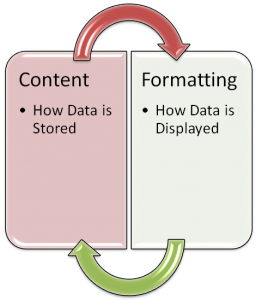
Many Excel Users are surprised to discover that the Delete Key does not clear the formatting for the selected cell or range of cells. This can cause some unusual “surprises” you you or one of your colleagues later uses this “Deleted” Cell Range!

On the other hand, some cells must be formatted properly in order to return the correct result. This is especially true for cells that contain Time and Date Calculations. For example, in order to properly calculate a Sum of Hours that exceeds 24 hours, you need to apply the Custom Format [h]:mm to the formula cell.

Topics Taught in this Tutorial

  • Adding the Clear Command to the Quick Access Toolbar (QAT).
  • Using Go To Special – Last Cell, to find the last cell in the worksheet that contains either content or formatting – or both!
  • Understanding how Excel Stores Dates (as a Serial Number) and Times (as a Decimal Number) vs. How you use Cell Formatting to make Dates & Times easier to understand.
  • Using Keyboard Shortcuts to add the Current Date – Ctrl + ; (semi-colon) or Current Time -Ctrl + Shift + : (colon), or to “Toggle” between Formulas and Displayed Results  -Ctrl + ~ tilde).

Visit My New, Secure Online Shopping Website

Stop by http://shop.thecompanyrocks.com to see the new products that I have created. You can also download – for FREE – my Chart of Popular Excel Keyboard Shortcuts when you visit.

Watch Tutorial in High Definition

Follow this link to view this Excel Tutorial in High Definition on my YouTube Channel – DannyRocksExcels

YouTube Tutorial for this Post

Share and Enjoy:
  • Add to favorites
  • Facebook
  • Twitter
  • Technorati
  • Print
  • email
  • Digg
  • StumbleUpon
  • del.icio.us
  • Yahoo! Buzz
  • Google Bookmarks
  • Orkut
  • SphereIt
  • Sphinn

How to Return Either an Approximate or Exact Match for VLOOKUP Function

Matches with VLOOKUP

Matches with VLOOKUP

One of my viewers asked me to explain – with examples – how and when to choose either an Approximate or an Exact Match using the VLOOKUP Function in Excel. .

Approximate Match for VLOOKUP

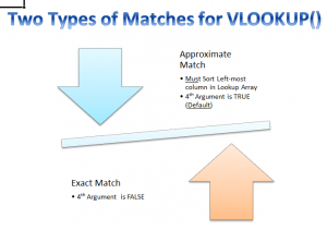
The Approximate Match is the Default setting for Vlookup. This means that you can either omit the 4th, optional, argument or use the word TRUE. However, as you will see in this video tutorial, there are other considerations to consider in order to get the correct result that you are looking for.

Exact Match for VLOOKUP

In the example that I use on the Video Tutorial, I am setting up an Employee Payroll worksheet. I definitely want to have an Exact Match for each employee to ensure that they are getting the correct amount of compensation for the hours that they worked during this period. Watch the tutorial to see how I set this up.

Watch Tutorial in High Definition

Follow this link to watch this Excel Tutorial in High Definition on my YouTube Channel – DannyRocksExcels

Get More Excel Tips

I invite you to visit my online shopping website – http://shop.thecompanyrocks.com – to preview the many resources that I offer. Here is the link to go directly to the information page for my DVD-ROM, “The 50 Best TIps for Excel 2007.”


Share and Enjoy:
  • Add to favorites
  • Facebook
  • Twitter
  • Technorati
  • Print
  • email
  • Digg
  • StumbleUpon
  • del.icio.us
  • Yahoo! Buzz
  • Google Bookmarks
  • Orkut
  • SphereIt
  • Sphinn

How to AutoFill the Letters in the Alphabet in Excel

 One of my viewers would like to be able to AutoFill the Letters in the Alphabet in his Excel Workbooks – he creates Alpha-Numeric Part Numbers for his products.

Two Ways to AutoFill Letters in the Alphabet

  1. Use a Formula – =CHAR(ROW(A65)) and AutoFill Down in the Column – This is not ideal
  2. Create and Use a Custom List in Excel. – So, use the Formula to create your list of 26 Alphabetical Letters. Copy the List and use Paste Special Values to convert the formulas to values. Then create your Custom List.

Using the CHAR() Function in Excel

There are 255 ASCI Characters that you can use in Formulas. For example, =CHAR(169) will return the © Symbol. In this lesson, I share a great Keyboard Shortcut that you can use to add this Symbol into the Footer of your printed Excel worksheet – Watch the video to discover this!

Visit My Secure Online Shopping Site

I hope that you take a few minutes to visit my new, secure online shopping website. The address is: http://shop.thecompanyrocks.com


Watch Tutorial in High Definition

On my YouTube Channel – DannyRocksExcels – I have posted this tutorial in High Definition Mode. Click here to go directly to this video.


Share and Enjoy:
  • Add to favorites
  • Facebook
  • Twitter
  • Technorati
  • Print
  • email
  • Digg
  • StumbleUpon
  • del.icio.us
  • Yahoo! Buzz
  • Google Bookmarks
  • Orkut
  • SphereIt
  • Sphinn

How to Use the Offset Function Inside a VLookup in Excel

Vlookup in Excel

VLOOKUP in Excel

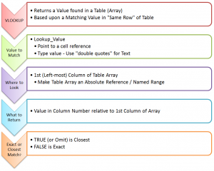
Each month, I get 5 to 6 emails of phone calls from viewers who who are having trouble using the VLOOKUP Function in Excel. In the majority of cases, the problem is that their Data Table is setup so that the “Key” field that they need to search in is NOT the Left-most or first field in the table. It is not always practical – nor desirable – to use “Cut and Paste” to rearrange the fields in the data set. So, what techniques can you use to fix this?

Use the OFFSET Function Inside a VLOOKUP Function

In this scenario, our IT Department sends us a daily report of the products that we sell including fields for the current cost and quantity on-hand. We use this report to generate additional reports and filters. This report gets saved automatically as an Excel 2010 Table with the name “Inventory.” The problem is, whenusing a VLOOKUP, that the first – or Left-most – field is NOT the “Key” field that we want VLOOKUP to use to search for a Match in order to return the current price or inventory for individual product.

The OFFSET() Function in Excel, makes it easy to reference a “starting field” that, in this case, is one column to the Right. This is perfect for our situation. We can continue to use our “named range” with the VLOOKUP!

Watch Video in High Definition

Follow this link to watch this tutorial in High Definition on my YouTube Channel – DannyRocksExcels

Visit My New Secure Online Shopping Website

I invite you to visit my new online shopping website at: http://shop.thecompanyrocks.com I have created new, extended length video tutorials that you can either purchase to download immediately or order them on a DVD-ROM. In addition, I have published versions of my 90 minute Pivot Tables Video Tutorials for Excel 2003, Excel 2007 and Excel 2010. So, I have the tutorials that you want for the Excel version that you are currently using!

Click to Play Excel Video Tutorial

Share and Enjoy:
  • Add to favorites
  • Facebook
  • Twitter
  • Technorati
  • Print
  • email
  • Digg
  • StumbleUpon
  • del.icio.us
  • Yahoo! Buzz
  • Google Bookmarks
  • Orkut
  • SphereIt
  • Sphinn

Structured Formula References in Excel 2007 and Excel 2010 – Part 2

Compare Structered References Excel 2007 v 2010

Compare Structured References 2007 v 2010

This is the second and concluding part of this series where I demonstrate how to use Structured Formula References when referring to Excel Tables.

Key Points Covered

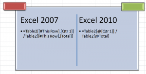
  • The difference between Structured Formula References in Excel 2007 and Excel 2010
  • How to Edit Structured Formula References
  • How to Write Structured Formulas using the new Formula AutoComplete drop-down menu


Watch My Video Tutorial Now


Watch Video in High Definition on YouTube

Click on this link to watch this Video in High Definition on my YouTube Channel – DannyRocksExcels

Go to Part 1 in this Series of Video Tutorials

Follow this link to go to Part 1 in this Series of Tutorials about using Structured Formula References in Excel Tables.

Visit My New Secure Online Store

I have just published 6 New Products and opened a new, revised, secure online shopping website. Take a look at: http://shop.thecompanyrocks.com


Share and Enjoy:
  • Add to favorites
  • Facebook
  • Twitter
  • Technorati
  • Print
  • email
  • Digg
  • StumbleUpon
  • del.icio.us
  • Yahoo! Buzz
  • Google Bookmarks
  • Orkut
  • SphereIt
  • Sphinn

How to Use Structured Formula References for Tables in Excel 2007 and Excel 2010

Structured Formula Reference - Excel 2007

Structured Formula Reference - Excel 2007

Beginning with Excel 2007, you can – and should – convert a Standard Data Range to an Excel Table. Doing so offers several advantages:

  • You get a selection of Table Styles – including Alternate Row Shading – that make it easier to read your tables.
  • You can automatically extend the Scope of your Table – by adding additional Fields (Columns) or Records (Rows).
  • You can give your Table a “Name” to reflect the purpose of the Table.
  • You can add a Total Row to Subtotal each Field (Column) and you can change the Function used to Subtotal from a drop-down menu.
  • You can apply Structured Formula References in the Table – Enter the Formula in a Single Cell and it is Automatically copied down for each record in the Table.

“In This Row” Formula Styles

Structured Formula References use a new style of formulas. Rather than referring to a specific Cell, in an Excel Table, you refer to a Field “in this row.” This type of formula is easy to create “inside the table.” It is also fairly easy to create “outside the Table” using the new Formula AutoComplete tool. You will be using [ ] (Left & Right Brackets) for these formulas. I go over these details, in-depth, in this video tutorial.

There are also distinct differences in how Structured Formula References are created between Excel 2007 and Excel 2010. These Structured Formula References are greatly streamlined in Excel 2010 – in my opinion.

The SUBTOTAL() Function and Excel Tables

I strongly recommend that you become familiar with how to use the valuable SUBTOTAL() Function in Excel when referring to the data in a Table. With the SUBTOTAL Function, you can produce a wide range of summaries anywhere on your Excel Workbook. And… the Subtotal Results reflect the totals for any “Filters” that you apply to your Table.

Play this Video in High Definition

Watch this Video in High Definition

Follow this link to watch this Excel Tutorial in High Definition on my YouTube Channel – DannyRocksExcels

Go to Part 2 in this Series of Tutorials

Follow this link to go to Part 2 in this series of tutorials about using Structured Formula References in Excel Tables.

Announcing 6 New Products on My New Online Secure Shopping Website

I invite you to visit my new online shopping site. I have added 6 new products – Extended Length Video tutorials that you can either “download now” or purchase as a DVD-ROM. Each product contains over 90 minutes of in-depth video instruction for Pivot Tables. You can choose the product to fit your version of Excel – Separate products for Excel 2003, Excel 2007 and Excel 2010.

Click here to view my new products.

Share and Enjoy:
  • Add to favorites
  • Facebook
  • Twitter
  • Technorati
  • Print
  • email
  • Digg
  • StumbleUpon
  • del.icio.us
  • Yahoo! Buzz
  • Google Bookmarks
  • Orkut
  • SphereIt
  • Sphinn

How to Take Advantage of the Go To Special Dialog Box Options in Excel

Go To Special Options

Go To Special Options

In my opinion, the Go To Special Options Dialog Box offers some of the most useful tools in Excel!

Why?

Because,  you must…

Select Cells Before Performing an Action on these Cells

The “key” to understanding ANY MS Office or Windows Program is… You MUST select a single cell or a range of cells BEFORE you can perform an action on them – e.g. Formatting you selection, deleting your selection, editing your selection or auditing your selection.

Tips Presented in this Video Tutorial

  • Select cells with Comments – so that you can “format” these cells to make them easier to identify.
  • Select cells that contain Constant Numeric Values – so that you can easily “spot” cells that should – bu do not – contain formulas.
  • Select cells that contain Specific Types of Formulas – e.g. Text Formulas – to “audit” your formulas.
  • Find the “Last Cell” in your worksheet – the last cell that contains EITHER content OR FORMATTING – This can be an “eye-opener!” for you.
  • Select the cells that contain Data Validation – perhaps you failed to “validate” all of the cells in a range.
  • Select the cells that contain Conditional Formatting – perhaps your did not select ALL of the cells in a Range BEFORE you applied a Conditional Formatting RULE!
  • Learn how to select the “Visible Cells Only” before performing a copy and paste operation – especially helpful when copying the “collapsed cells” for an Excel Outline.

I am positive that Excel users at ANY LEVEL will be able to pick up at least one solid tip from this Video Tutorial. Please send me your comments to let me know what you learned – or what you need clarification on.

Watch Tutorial in High Definition Mode

Follow this link to view this Excel Tutorial in High Definition / Full Screen Mode on my YouTube Channel – DannyRocksExcels

Learn About My New Extended Length Excel Video Tutorials

I have just published the first in a series of “Extended Length” – 90 Minutes – Video Tutorials, “Excel Pivot Tables to Summarize, Analyze and Present Your Data.” Follow this link to learn more about this tutorial. I have created separate versions of the tutorial for Excel 2010, 2007 and 2003.

Share and Enjoy:
  • Add to favorites
  • Facebook
  • Twitter
  • Technorati
  • Print
  • email
  • Digg
  • StumbleUpon
  • del.icio.us
  • Yahoo! Buzz
  • Google Bookmarks
  • Orkut
  • SphereIt
  • Sphinn