Learn How Excel Calculates Formulas

Order of Calculations in Excel

Excel Calculation Order

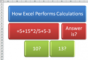
Have you ever written a Formula in Excel only to receive a result that was different from the one you expected? Most Excel users have shared that experience from time to time! Excel is smart and fast. However, it can not read your mind.

In this lesson, I show you how Excel evaluates and calculates a formula. Once you understand “Excel’s perspective” of the formula, you will know how to correctly write the formula so that Excel will produce the result that you intended. In other words, to see the formula from “your perspective!

Order of Precedence

Excel performs calculations in formulas moving from left to right in this order:

  1. Performs Multiplication (*) and Division (/)
  2. Goes back and performs Addition (+) and Subtraction (-)

This is the “key” to consistently getting Excel to produce the results that you intended. No, you can’t get Excel to make you an “instant millionaire” or do anything illegal. However, understanding how to write formulas correctly – so that you control the order of calculation in Excel – is the “secret sauce!”

Control the Order of Calculation in Excel This formula: =5+15*2 results in 35. If you were expecting the result to be 40, then write the formula as (5+15)*2. In other words, take the “result” of 5+15 or 20 and multiply this by 2 to give me 40.By using parentheses (5+15) you take control over the order of precedence that Excel uses. Help Excel to see the formula from your perspective!

Free Chart of Excel Formula Operators

I have published  a chart – “Using Operators in Excel Formulas” – To get your free copy as a PDF, click on the link below:

CR – Using Operators in Excel Formulas

Explore My Free Excel Video Lessons

Follow this link to my Index of Free Excel Video Tutorials

Watch This Video Tutorial In High Definition

This link will take you to the DannyRocksExcels video on YouTube
When to Use Absolute, Relative & Mixed Cell References in Formulas

In my experience, I find that many Excel users get easily confused when it comes time to use an Absolute or a Mixed Cell Reference in a formula. Let me demonstrate how and when to use the proper cell references, so that you always get the correct result.

Here is what each type of cell reference looks like in a formula:

  • Relative Cell Reference – =A2*B2 when copied down one row becomes = A3*B3
  • Absolute Cell Reference – =A2*$B$2 when copied down one row becomes =A3*$B$2 (Notice the $B$2 Absolute cell reference in the formula)
  • Mixed Cell Reference – =$A2*B$3 when copied down one row becomes = $A3*B$3 and when copied one cell to the right becomes =$A*C$3 (Notice how one part of the cell reference is relative – it moves; and the other part of the reference is Absolute – it remains fixed in place)

Learn how to “Master Excel in Minutes – Not Months!”

How to reveal the formulas in all cells

Here are the steps to follow for this lesson:

  1. To reveal the formula in a single cell, double-click the cell or press the F2 key.
  2. To reveal all of the formulas in the worksheet use Ctrl + Tilde (Ctrl+˜) – This is a “toggle.”
  3. There are 4 ways to write a formula to show the discounted price:
    1. If the cell containing the discount % is a negative (-20%) number =B5+(B5*$D$2)
    2. If the cell containing the discount % is a positive (20%) number =B5-(B5*$G$2)
    3. If the cell containing the discount % is a negative (-20%) number =B5*(1+$D$2)
    4. If the cell containing the discount % is a positive (20%) number =B5*(1-$G$2)

Find the video lesson that you want – Index to all Excel Topics

News! My DVD, “The 50 Best Tips for Excel 2007” is now available to purchase. I invite you to visit my online bookstore for more details.

Related Videos