Archives for 2010

Working with Multiple Worksheets in Excel

The 50 Best Tips

The 50 Best

In this video lesson, I share my tips for maintaining a consistent look when working with multiple worksheets in Excel. I will demonstrate how to:

  • Group multiple worksheets for editing
  • Make a copy of an Excel worksheet
  • Use the Fill Across Worksheet tool – to update Contents or Formats or Both – for a Group of worksheets

In a professional setting, it is important to make a consistent presentation of your Excel worksheets. You want each worksheet in the group to use the same formatting styles, headers and formulas. The tips that I demonstrate will definitely save you time and help you to maintain a consistent look.

Click here to watch this video in High Definition, Full Screen mode on my DannyRocksExcels YouTube Channel.

Learn how to “Master Excel in Minutes – Not Months!”

Invitation to Visit My New Secure Online Shopping Site

I have just opened my new, secure online shopping website. I invite you to visit http://shop.thecompanyrocks.com to see the new products that I have introduced in the year 2011.

Learn How to Use Date Functions in Excel

Excel has a group of functions that help you to calculate dates. For example, the number of days between two dates or the date on which an invoice will be payable.

This is the second in my series of lessons where I demonstrate how to enter and calculate dates and times in Excel. Here is the link to part one.

Excel Tip List

Excel DVD Tips

The date functions that I demonstrate on this video are:

  • TODAY()
  • NOW()
  • DATE()
  • DATEVALUE()
  • WORKDAY()
  • NETWORKDAYS()
  • EOMONTH()

The last three date functions require you to activate the Analysis ToolPak Add-in. You will also learn some valuable and time saving keyboard shortcuts.

You can watch this video in High Definition, Full Screen Mode on my YouTube Channel – DannyRocksExcels

Learn how to “Master Excel in Minutes – Not Months!”

How to Work with Dates in Excel

The majority of the questions that I receive from viewers center on how to use and format DATES & TIMES in Excel. So, I have decided to create a series of lessons to show you how to work with dates and times in Excel.  This is part one in a continuing series of free Excel Video Training Lessons.

50 Best Tips for Excel 2007

Excel Tips

Learn How to Work with Dates

  • Use a Keyboard Shortcut to enter the current date in a cell – to “time stamp” the date.
  • Use the TODAY() Function to enter a “dynamic” date function in a cell – so that your date always reflects the current date.
  • Distinguish between how Excel “stores” a date – as a serial number – and how Excel formats a date – how you choose to format a date.
  • Tell if a date was entered correctly – as a number – or incorrectly – as “text” by seeing how it is aligned in the cell (right or left).
  • See why a fraction could be recognized as a date – and how to correct this “got’cha” step!
  • How to create a series of dates in your spreadsheet.

In my experience, the majority of “Excel problems” are based around incorrect date and time entries. So, whether you are new to Excel or a veteran who gets frustrated with Time and Date calculations, this lesson is for you.

If nothing else, you will pick up some great Keyboard Shortcuts in this lesson!

Follow this link to watch this video in High Definition, Full Screen Mode on my YouTube Channel – DannyRocksExcels

Learn how to “Master Excel in Minutes – Not Months!”

Use the SUMPRODUCT Function to Total Lists Using Multiple Criteria

In Excel 2007 and Excel 2010 you can use the new SUMIFS Function to total a list using multiple criteria. This is a great new feature!

But … what if you are using Excel 2003 or earlier? Or, if you collaborate with colleagues and clients who use older versions of Excel – how can you use multiple criteria to select the records that you want to Sum? You can use the SUMPRODUCT Function as I demonstrate in this video lesson.

The 50 Best Tips

The 50 Best Tips Series

Key Concepts

  • Create – and use – Named Cell References for Ranges / Arrays in your formulas
  • Use the Function Arguments Dialog Box – Use the keyboard shortcut Ctrl + A to bring this up
  • Use the F3 Keyboard Shortcut to bring up the Named Ranges List
  • In this lesson, use () to enclose each Array Argument
  • In this lesson, use * to substitute for the , to separate each Array in the formula (Edit this in the Formula Bar)

There are usually several ways to solve any problem in Excel. This is a good procedure to learn – regardless of the version of Excel that you use.

Click here to view the 1st part of this series on how to use the SUMPRODUCT Function in Excel.

You can view this Excel Video in Hig Definition, Full Screen Mode on my YouTube Channel – DannyRocksExcels by clicking here.

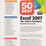
I cover the SUMIF and SUMIFS Functions in greater detail on my DVD, “The 50 Best Tips for Excel 2007.” Click here to start shopping using my secure shopping cart.

Learn how to “Master Excel in Minutes – Not Months!”

How to Use the SUMPRODUCT Function in Excel

In my experience, most Excel users are unfamiliar with the SUMPRODUCT Function. So let me give you two reasons to watch this short (5 minutes, 22 seconds) video lesson to learn how – any why – to use SUMPRODUCT:

  1. The SUMPRODUCT Function will speed up your calculations in Excel – get results with one step. With SUMPRODUCT() you can avoid several intermediary calculations.
  2. With SUMPRODUCT, you may be able to trim the size of your Excel worksheet. You may not need as many columns (fields) as you think to get the result that you need!

In this lesson, I show you how to calculate the Total Value of the Inventory (for a fictional company) with one formula!

50 Best Tips for Excel 2007

Excel Tips

Key Points Coverered

While the SUM Function “Adds Up” the values in the Arguments, the PRODUCT Function “Multiplies” the values in its Arguments.

  • Using “Arrays” in SUMPRODUCTS. In Excel 2007, you can use up to 255 Arrays! The key point is that all Arrays must be the same size and shape. For example, if the 1st arry in the Arguments is 15 rows in one vertical column, then all of the subsequent Arrays must be 15 rows in one vertical column.
  • I find that Creating – and Using – Names Cell Ranges for the Arrays will speed up writing the SUMPRODUCT formula.

I have decided to present the SUMPRODUCT Function in two lessons – so click on the sequel to see other uses for this function!

Click here to watch the 2nd video lesson on how to use the SUMPRODUCT Function in Excel.

You can watch this Excel Training Video Lesson in High Definition, Full Screen Mode on my YouTube Channel – DannyRocksExcels

You can learn how to “Master Excel in Minutes – Not Months!”

How to Speed Up Data Entry on Forms By Using Named Cell Ranges

You can speed up data entry on an Excel form by creating – and using – named cell ranges. This also improves data accuracy, because the data entry clerk only has to hit the “Enter” key after each imput; the curosor automatically moves to the next cell in the named range that you applied to your form!

There is one “got’cha” step in this process. As you will see in this video, it is important to observe the position of the “Active Cell” in your selection!

The 50 Best Tips

The 50 Best Tips Series

Key Points Covered

  • Hold down the “Ctrl” key as you click on the cells in your non-contiguous range.
  • Use labels and cell shading to identify the cells that require data input.
  • When selecting your non-contiguous cells, choose the cell that you want to be the “Active Cell” last.
  • You can enter a formula or value into all of the cells in a range with “Ctrl+Enter.”

Try this out  on a form that you use at work. Remember to create a “name” for your data input cells. “Named cell ranges” are saved when you create a copy of your workbook – so this technique can be easily duplicated by saving the file with a new name.

Click here to watch this video in High Definition, Full Screen Mode on my YouTube Channel – DannyRocksExcels

Learn how to “Master Excel in Minutes – Not Months!”

How to Name a Large Range of Non-Contiguous Cells in Excel

A client asked for my help on this problem. How to create a Named Range in Excel for Non-Contiguous Cells. The problem is that Excel puts a 255 character limit on the “Refers to” portion of a Named Range. I struggled with this until I found the answer in one of my favorite resource books, “This isn’t s Excel, it’s Magic!” written by Microsoft MVP (Most Valued Professional) Bob Umlas.

Solve the Problem

  1. Select the non-contiguous cells that you want to name.
  2. Open up the Visual Basic Environment (Alt + F11 is a Keyboard Shortcut).
  3. In the VBE, open up the “Immediate Pane” – Ctrl + G is the Keyboard Shortcut.
  4. Finally, type Selection.Name = “MyLabels” in the Immediate Pane and press Enter. (Substitute the name you want for “MyLabels”).

When you return to Excel, you will see that you can use the Drop-down list in the Name Box or in the Excel 2007 Name Manager to select this range.

 Amazing! Thanks Bob!

Additional  tips

  • Keyboard Shortcut F5 to open up the “Go To” Dialog Box. Select “Special” and choose “Constants – Text” to select the non-contiguous Labels that you want to name.
  • Right-click the worksheet tab and select “View Code” top open up the VBE (Visual Basic Environment) window.

I invite you to watch and subscribe to my Video Podcast on iTunes – follow this link to “Danny Rocks Tips and Timesavers”

Click here to watch this video in High Definition, Full Screen Mode on my YouTube Channel – Danny Rocks Excels

Learn How to “Master Excel in Minutes – Not Months!”

My Most Viewed and Downloaded Videos for Excel and PowerPoint

My iTunes Podcast

Danny on iTunes

I began to post my videos as podcasts at the iTunes store this past summer. Since then, my video lessons for Excel and PowerPoint have been viewed and downloaded many times. I am thirlled. And, I thank you for your support and encouragement.

Here are the links – on my website – to the most popular video episodes. I have organized them by category in the order of their popularity. You can click on any link to view or download that video from my website. Or, you can go to my video Podcast by clicking on this link – “Danny Rocks Tips and Timesavers” Podcast on iTunes.

Merging and Consolidating Excel Worksheets

 PowerPoint Presentations

Data Visualizations

What-If Analysis in Excel

Importing Data From Other Programs

Pivot Tables

Excel Tables

Social Media

Formula Errors

Please add your comments below – or on my iTunes Channel. I welcome your feedback.

You can learn how to “Master Excel in Minutes – Not Months!”

Sincerely,

Danny Rocks

How to Annotate Excel Worksheets with Comments and Images

Do you use “post-it” sticky notes to remind you how to do something? Do you ever lose your reminder notes? I know that I do! So that is why I like to annotate my Excel Worksheets with Comments – this way I have the notes properly located (in the worksheet) when I need them (to remember how to write a particular formula, etc.) the most!

In this lesson, I also show you how to add “pictures” inside your comments. This is a great tip for adding in a picture for a catalog or order form.

A question that I am frequently asked: “How do I print out my comments?” Watch this video to find out how to do this – there are a couple of “got’cha” steps involved.

Logo for The 50 Best Tips

The 50 Best Tips

Here are three ways to enter a new comment that is attached to a single cell:

  • Use the Keyboard Shortcut Shift + F2
  • Right-Mouse Click and choose “Insert Comment”
  • On the Review Tab of the Ribbon (Excel 2007) select the “Insert New Comment” command.

You can edit your comments, re size the shape of your comments, hide your comments (only a “red triangle” shows in the cell until you hover near the cell), show your comments (individually or collectively), delete, clear and paste your comments. I cover each of these techniques in this video lesson. And more!

Watch this video in High Definition, Full Screen Mode on my YouTube Channel – DannyRocksExcels

Learn how to “Master Excel in Minutes – Not Months!”

Watch My Excel Videos in High Definition Full Screen Mode on YouTube

Logo for YouTube

YouTube Logo

At the request of several viewers, I have begun to produce my Excel, PowerPoint, Word, Outlook and Access Video Lessons in High Definition, Full Screen Viewing Mode. You can watch them, download them, share them and comment on them on YouTube. My YouTube Channel is DannyRocksExcels.

Here is the link to the YouTube”Playlist” that I have created for the HD Videos:

http://www.youtube.com/view_play_list?p=9D34C8C834E21A51

Please “bookmark” this link. As I add more HD Videos on YouTube, the Playlist will be updated.

My iTunes Podcast

Danny on iTunes

I will continue to post my videos on www.thecompanyrocks.com in M4V video format so that they can be sent automatically to the iTunes store. I invite you to subscribe to my video podcast – Danny Rocks Tips and Timesavers – on iTunes. It is free! Here is the link to my iTunes podcast:

http://itunes.apple.com/podcast/danny-rocks-excel-tips/id374923275

I welcome your feedback on my videos. Let me know what you like, what you don’t like or would like to see improved. Send me your questions and I will do my best to answer them promptly. Just drop a note to say hello!

Learn how to “Master Excel in Minutes – Not Months!”