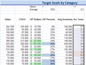
Use Conditional Formatting in Excel to Highlight Cell Values that Match Criteria

Conditional Formatting in Excel

Conditional Formatting has been available for many years in Excel. However, beginning with Excel 2007, Conditional Formatting got a major boost in its ease-of use and new visualization tools.

In this tutorial, I demonstrate how to use Conditional Formatting to highlight – via formatting – the cells in a range that anser “TRUE” to a set of criteria. For example, is the cell value “Above Average” or is it Greater than the value in a Target Cell.

How Does Conditional Formatting Work?

Conditional Formatting is “dynamic.” If you update the values – or formulas that generate cell values” the cell that receive the Conditional Formatting may change – based upon the criteria that you set as “the condition.”

Versions of Excel Covered

For this lesson, I demonstrate Conditional Formatting in BOTH Excel 2010 and Excel 2003.

Learn More About Conditional Formatting

I invite you to visit my secure online shopping website – http://shop.thecompanyrocks.com – to see all of the resources that I offer. This includes my best-selling DVD-ROM, “The 50 Best Tips for Excel 2007.”