How to Take Advantage of Report Filters in Excel Pivot Tables

Starting with Excel 2007, Pivot Tables now include a “drop field” labeled “Report Filters.” The Report Filters area replaces the area labeled the “Pages” drop area in Excel 2003 and earlier. Report Filters is a more descriptive and intuitive name. So , this is a welcome change.

How to Organize Pivot Table

Use Report Filters in Pivot Table

In this lesson, I am responding to an additional request from one of my viewers who wants me to demonstrate how the “Report Filters” drop zone will provide incredible reporting power in a Pivot Table.

Request from a Viewer

In this lesson, my viewer is a “hydrologist” who analyzes average Water Flows by day and by month in a “Water Year.” If you use a “Fiscal Year” reporting structure, you will want to pay attention to this lesson. In this case, the “Water Year” begins on October 1 and ends on September 30. My viewer needs my help in separating out individual Pivot Table Reports organized by Water Year – placed in the Report Filters Drop Zone.The Pivot Tables show the average daily water flow by date. He told me that he is concrned that that Pivot Table Report may not be able to “account for Leap Years.”

Not to worry!

Watch this Excel Video Tutorial, as I demonstrate how to answer my viewer’s query and also give you some “solid tips” to get the results that you need when using Excel!

Watch this Excel Video Tutorial in HD Mode on my YouTube Channel

Here is the link to my YouTube video channel for this video.

Learn how to “Quickly Create Pivot Table Reports!”

Create a Pivot Table for a Water or Hydrological Year

A viewer asked for my help in creating a Pivot Table Report that is based on a Water Year – also known as a Hydrological Year. In North America, a Water Year begins on October 1 and ends on September 30. If you use a Fiscal Year in your reporting, you will want to watch this Excel Training Video Lesson.

Pivot Table for Water Year

Pivot Table for Water Year

Add Two Fields to Source Data

In order for a Pivot Table to summarize non-calendar years and quarters you will need to have two additional fields in your source data:

  1. A Fiscal Year (Water Year) Field – Use the IF(), MONTH() and YEAR() Functions to produce this.
  2. A Fiscal Quarter (Hydrological) Quarter Field – Use the CHOOSE() Function to produce this.

Now you are ready to create your Pivot Table Report.

Group Dates by Month and Year

Begin by grouping the Date Field by Month and Year – not, in this case, by Quarter. Now, remove the new Year field that you just created and add in the Water Year Field and the Hydrological Quarter to the Pivot Table. Continue to arrange the Pivot Table to suit your needs.

Since there is no direct way to change a Calender Year into a Fiscal Year or Water Year, you must prepare your data prior to beginning to create your Pivot Table. Now that you have watched this video lesson, you know how to do this!

Learn how to “Quickly Create Excel Pivot Tables and Charts”

Related Excel Video Lessons

Follow this link to watch this video in High Definition mode on my YouTube Channel – DannyRocksExcels

How to Use Date Functions and Date Formatting in Excel

In this lesson, I respond to two recent requests from viewers for help in Using DATE Functions in Excel and also, how to apply Custom Date Formatting. I get similar requests on a frequent basis from both viewers and clients.

Solve Problem #1 

My first viewer wants help in using the DATE() Function in Excel. She wants to calculate a date that is 90 days after the starting date for a project. She encountered two problems

  1. Initially, the DATE() Function produced and error – because she forgot to ‘nest” the YEAR(), MONTH()+9, DAY() Functions inside the DATE() Function.
  2. She was not expecting a date to be filled in the formulas column when there was no starting date for the project – She needed to include an IF() function to perform a LOGICAL TEST – Does  the Starting Date = 0, Value if TURE, ” ” (to display nothing), Value if FALSE – to perform the calculation.
Excel Custom Date Formats

Excel Custom Date Formats

Solve Problem #2

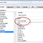
My second viewer wanted my help to ensure that the date values that he “pasted” into a range of cells were in the (Custom) format of “yyyy-mm-dd” (Year, Month, Date).

In this case, we need to take two steps:

  1. Format the destination cells using the CUSTOM FORMAT of yyyy-mm-dd that we create.
  2. After “Pasting” the Copied Cells, use the “Paste Options” dialog box to select – “Match Destination Formatting.”

I also demonstrate how to use the NETWORKDAYS() Function and the WORKDAY() Function – with an optional list of “Holidays” to exclude. And, finally, I show you the “pitfalls” that occur when you import a “text” file of dates that use a variety of formats. In order to perform DATE calculations, a date must be stored as a NUMBER in Excel. It must be right-aligned in the cell.

You can watch this Excel Video Lesson in High Definition, Full Screen Mode on my YouTube Channel – DannyRocksExcel – by clicking this link.

Learn to “Master Excel in Minutes – Not Months!”