Create User Friendly Excel Forms Using Spin Button Controls

An Excel Form is great way to distribute an Excel worksheet to your customers or field representatives. Most of the time, you do not want them to type values into a cell. You want to make this Form as “user friendly” as possible! You want to add “Spin Buttons” to your form, so that the user can simply click to change cell values up or down in the increments that you want to display.

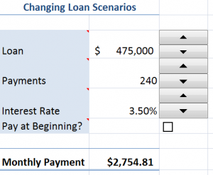
A perfect example: A Mortgage Loan Scenario where – by clicking the Spin Buttons – your client can see what their monthly payment will be. This is my second lesson covering Excel’s Form Control Tools. Watch as I demonstrate how to “work around” the Form Controls limits of Maximum Amount for a Spin Button (30,000) and also how to increment interest rates by 1/4 of a Percent.

From personal observation, I know that many people start to create an Excel Form and then just give up in frustration. I did too – in the beginning! Watch me demonstrate how to avoid the traps of the “got’cha” steps in this short Excel Training Video.

Check out the great tips that I offer on my DVD, “The 50 Best Tips for Excel 2007.” Click here to start shopping.

Learn how you can “Master Excel in Minutes – Not Months!”

How to Add a Check Box Control to an Excel Form

Judging by the comments that I get from many clients, adding a “Check Box Control” to and Excel Form is not as easy as it appears at first glance.

And, I agree! I, too, struggled with adding Form Controls in Excel. Most of the explanations that I read seemed to add more confusion than clarification!

Spin Buttons in Excel

Spin Button Controls

That is why I created this Excel Training Video: to  lead you through the process; to save you some time and to ease your frustration.

Key Points to Remember:

  1. In Excel 2007, be sure to display the “Developer Tab” on the Ribbon in order to to Insert any Form Control.
  2. Choose the Controls in the “Forms Controls” and NOT in the Active X Controls.
  3. After you “draw” the Control Box on your Form, be sure to select a “Cell Link” to enable the Check Box Control.
  4. Remember that a Check Box Control can only be applied when the result of the Formula or Option is a Logical Value – either a result of  “True or False.”

Don’t be scared off! I find that this is an Excel concept that is better presented “visually.” I struggled for some time when I “read” how to add form controls.

So … I welcome your thoughts – “True or False.” Did I make this easy for you to understand?

Please feel free to add your comments below!

Watch My Video on YouTube

Follow this link to watch my tutorial on my YouTube Channel – DannyRocksExcels

Watch Video Now


Master Excel in Minutes Training Resources

I have created a series of extended length Excel Training Videos. I invite you to visit my secure online shopping site to:

Learn how to “Master Excel in Minutes – Not Months!”

Excel Tells You the Future Value of Your Investment

Hey, want to know what your investment will be worth in 5 years? 10 years? Want a sure thing? Excel correctly calculates the future value of any investment! Provided …

  • You make a series of regular investments – even if it is just one “lump sum.”
  • The interest rate that you earn is “constant” – that is a “fixed annual interest rate.”

OK, so now you understand that neither I nor Excel are “touting sure thing” winners in the stock market. No one can do that. But, you can’t beat Excel when it comes to accurate – and easy to use – financial calculations.

In this video lesson, I demonstrate how to use both the =FV() and =PMT() Functions to calculate Future Values. I also show you how to perform “What-If” Analysis using a One-Input Data Table.

Here are the steps to follow in this Excel Video Lesson:

  1. Input values for Interest Rate (RATE), Number of Periods (NPER) and your Investment (PMT). These are the three required arguments for the =FV() Function. Use the Function Argument Dialog Box to ensure that you use the correct syntax for this function.
  2. One of the “optional” arguments is “Type.” If you omit this, Excel defaults to a “0” which means that you will make your investment contribution at the end of each period. A “1” means that the contribution is made at the beginning of each period. Over a number of years, this can make a significant difference in the “Future Value” of your investment.
  3. FV is also an “argument” in the =PMT() Function. If you want to calculate how much you need to contribute each month to reach a Savings Goal, use the =PMT() Function. However, in this case, the FV – while showing as an “Optional Argument” will refer to the cell containing your Savings Goal.
  4. Create a One-Input Data Table to perform “What-if” Analysis – e.g. to substitute a series of different interest rates in your =PMT() – or =FV() Function.

NEW! Download the Practice File for this Excel Video Lesson:

Find the Excel Video Lesson you want – Index of all Excel Topics

News! My DVD, “The 50 Best Tips for Excel 2007” is now available to purchase. I invite you to visit my online bookstore for more details.

Perform "What-if" analysis with a 2 input Data Table

Here are the steps to follow in this video lesson:

  1. Create a formula that references cells – e.g. =PMT(B4/12,B5,B3)
  2. To the right of this formula cell, enter a series of “substitute” values – e.g. 36, 48, 72 months.
  3. Directly below the formula cell, enter another series of “substitute” values – 4%, 4.5%, 5%, etc.
  4. Select the range of cells for the Data Table – starting with the formula cell.
  5. From the Excel Menu, choose Data, Table.
  6. For the “Row Input Cell,” click the cell in the original formula for which you want to “substitute” the row values in your Data Table.
  7. For the “Column Input Cell,” click the cell in the original formula for which you want to “substitute” the column values in your Data Table. Then click OK.

NEW! Download the Excel Workbook that I Use in this Video:

Find the video lesson that you want – Index to all Excel Topics

News! My DVD, “The 50 Best Tips for Excel 2007” is now available to purchase. I invite you to visit my online bookstore for more details.

Goal Seek to optimize the results of the =PMT() function

Here are the steps to follow in this video lesson:

  1. Calculate your monthly payment on a loan using =PMT() function
  2. =PMT() requires three arguments: “Interest Rate” / # of payments per year, “# of payments” over the course of your loan, the “Amount Borrowed.”
  3. For Goal Seek: Select the cell that contains your formula and then choose Tools – Goal Seek.
  4. In the “To Value:” box type in your GOAL – e.g. The amount that you want your =PMT() to return.
  5. In the “By Changing Cell:” select a cell that is referenced in your =PMT() formula.

Find the video lesson that you want – Index to all Excel Video Lessons

“The 50 Best Tips for Excel 2007” DVD is now available to purchase. I invite you to visit my online bookstore for more details.