Master Excel Pivot Tables in 90 Minutes: Announcing My New Extended Length Video Tutorials!

Master Pivot Tables in Minutes

Master Pivot Tables in Minutes

I am proud to announce the publication of my new series of “Extended Length” video tutorials: “Master Excel Pivot Tables in 90 Minutes!”

Now, you can can get an in-depth video tutorial, so that you can Master Excel Pivot Tables with 90 minutes of video instruction. You also receive the actual Excel Workbook file that I used while filming the video lessons as well as a printed step-by-step instructional manual.

What Makes this Product Unique?

  •  Excel Versions for the Video Tutorials

  • Available for Excel 2010, Excel 2007 or Excel 2003

Multiple Options for Delivery

Resources to Assist Your Learning

  • The Excel Workbook file that I used while filming each video lesson – Included with purchase!
  • PDF Manual of Step-by-Step Instructions – That you can print out – Included with purchase!

Take a Short Video Tour

Follow this link to watch a short – 5 minutes – video tour of my new products on my YouTube Channel – DannyRocksExcels

Visit My New Secure Online Shopping Website

I invite you to visit http://shop.thecompanyrocks.com This is my new online shopping website. I have created secure shopping carts to ensure that your privacy is protected. I also offer a 100% Customer Satisfaction Policy. If, for any reason, you are not 100% satisfied with any of my products, I will refund your purchase with no questions asked!

Danny Rocks

The Company Rocks

Create a Pivot Chart to Present a Frequency Distribution Report

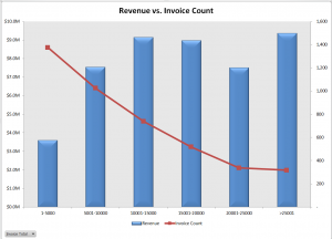
Combination Chart for Frequency Report

Quite a few of my viewers requested that I continue my series of creating and presenting a “Frequency Distribution Report” using an Excel Pivot Table. So, here is the new Part 3 in the series!

In this Excel Video Tutorial, I demonstrate – using Excel 2010 – how to create a Pivot Chart for the Frequency Distribution Pivot Table that I created and modified in Parts 1 and 2 of this series.

Key Point: A Pivot Chart Must be based on a Pivot Table Report!

  • Any structural changes that you make to the Pivot Table are reflected in the Pivot Chart.
  • If you “filter” the Pivot Chart, those filters apply to the Pivot Table that is the basis for your Pivot Chart – and vice versa.

Focus on the Chart

As I demonstrate in this video – posted on YouTube – I prefer to focus on one task at a time. I prefer to get the formatting and structure of the Chart “right” before I think about using Filers and other “goodies to add .” This “Best Practice” helps me to get more accomplished in less time!

My bottom line is: “Focus on the task at hand. Eliminate any possible distractions from that primary task!”

A correctly designed Pivot Chart will help you to present your information accurately and interactively! For this presentation, I decided that a “Combination Chart” would be the best way to present the information that I wanted to convey. A “Combination Chart” allows you to have a Primary Axis (Revenue) that uses a Column Chart Type and a Secondary Axis (Invoice Count) that uses a Line Chart Type.

When to Use a Secondary Chart Axis

In this example, there is a wide difference between the two fields that we are charting:

  • Revenue for the Invoices in the “Bin Range” is in “the millions!
  • Count of Invoices in the “Bin Range” falls into the hundreds and low thousands.

Using a “Combination Chart” in this example – (Column Chart for Revenue in Millions) and Count of Invoices (Line Chart for Count in Hundreds) allows you to present the “relationship” between both metrics. I show you step-by-step how to create this combination chart!


Watch This Video in High Definition on YouTube

Follow this link to view this video tutorial in High Definition on my YouTube Channel – DannyRocksExcels

Click this link to view Part 1 of the 3 Part series – Creating a Frequency Distribution  Report with Excel Pivot Table

Click this link to view Part 2 of the 3 Part series – Formatting a Frequency Distribution Report with Excel Pivot Table

My Extended Length Pivot Tables Video Recordings Available for Excel 2003, 2007 and Excel 2010

On my WebEx site – http://thecompanyrocks.webex.com – I have posted three, one-hour-plus video recordings to help you to learn how to create and customize Excel Pivot Tables:

Download “Free of Charge” Resources for Each Recording

Click on the hyperlinks above to go to a special landing page for each Excel version. From the landing page, you will find links to download the resources that accompany each version:

  • The Excel Workbook – in each version of Excel (2003, 2007, 2010) that I use during the video recording.
  • The Step-by-Step Instructional Manual that I created for each Excel version of my recordings.
    • Available as an Adobe Acrobat PDF or as a Word Document

Very Attractive Pricing for Recordings

I have decided to price each of these recordings – which you can download to your computer – at US$9.95

  • Imagine what you would have to pay to hire a trainer – per hour –  to teach you these Pivot Table lessons!
  • Imagine how many pages in a book you would have to wade through to read about Pivot Tables!
  • Now, imagine being able to:
    • Watch a video demonstration of the steps to take to create or customize a Pivot Table.
    • Read – and make notes in – a written document that follows the steps that I demonstrate.
    • Practice the techniqes that I demonstrate on the video with the actual Excel worksheets that I use.
    • Skip back and forth to the chapter that you want to watch or review on the video recording.
    • Download the recording for the exact version of Excel that you are using.
    • Get all of this for only US$9.95

What You Will Learn on My Video Recordings

I have taken care to organize each of these topics “by chapter” – with starting points and ending points – on the recordings:

  • Create a Pivot Table in the Excel version that you are using.
    • Spotlight the uniqe features of each version
  • Filter and Sort the Fields in your Pivot Table
  • Change the Data Source & Refresh your Pivot Table
  • Use Multiple Functions and Views to Calculate your Pivot Table
  • Create a Calculated (“virtual”) Field in your Pivot Table
  • Group Fields – e.g. turn daily transactions into a Month, Quarter, Year Pivot Table Report
  • Create and Filter Pivot Charts
Download WebEx Recording

Download WebEx Recording

Download My Recordings at WebEx

  • Go to http://thecompanyrocks.webex.com and on the left side of the screen click on “Attend a Session – Recorded Sessions” to find the recording that you wish to download.
  • Register and enter your payment information – this is a secure shopping site.
  • Download the recording – also download the WebEx Recording Player so that you can play the ARF recording.
    • I recommend that you “Save” your recording on the download page. Play it from your directory of choice after it has downloaded
    • From the ARF Player for the WebEx Recording, you can convert the recording to another video format (MP4, AVI, WMV or SWF)

I welcome your feedback. Send me your questions, comments and suggestions for future recordings.

Download My 75 Minute Video Tutorial on Excel 2007 Pivot Tables

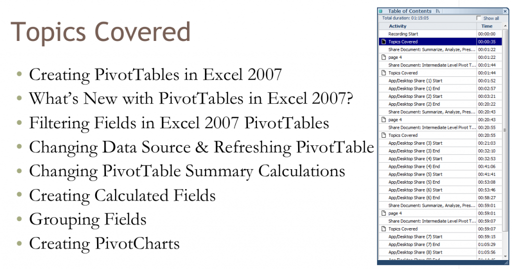
Topics Covered

Table of Contents for Recording

I have just recorded and published a 75 Minute Video Tutorial titled, “How to Create and Modify a Pivot Table in Excel 2007 to Summarize, Analyze and Present the Information in your Data Set.”

It is published on my WebEx by Cisco site: http://thecompanyrocks.webex.com Follow this link to go directly to this recording.

There is a charge for this recording – US$9.95 In addition to the recording you get:

  • A Step-by-step instructional manual
  • Access to the Excel workbook files that I used for this recording

Not to brag , but I think that this video tutorial is excellent! I spent many hours planning out the exercises, working through the timing of each chapter of the video and practicing my delivery. I am happy with the result. And, more important, I think that you will also be satisfied with what you will learn from this recording!

What You Will Learn on My Recording

My goal is to give you a comprehensive understanding of Excel 2007 Pivot Tables. But to give you the opportunity to learn this in “bite-size chunks” that can replay when necessary. I created realistic exercises to illustrate each topic.  Also notice that I have created a Table of Contents for the recording so that you can go to a specific chapter on the recording. You can stop and start at any point.

How to Download this Recording

  1. Go to http://thecompanyrocks.webex.com or click on this link to go to the main menu.
  2. Click on “Recorded Sessions.”
  3. Click the link for the recording, “Excel 2007 Pivot Tables to Summarize Data.”
  4. Register for this session (First Name, Last Name and email address).
  5. Enter payment information (PayPal or Credit Card). This is a secure site!
  6. Follow the instructions to Download my recording.
  7. Recommended – you can also download the ARF Recorder to view the recording.
  8. At this point you can decide to convert the recording to a different format. E.g. WMV (Windows Media Player), SWF (Flash) or MP4 (MPEG4)
  9. At the end of the recording, you are taken to a web page with links to download the Instructional Manual and to download the Excel Workbook that I used during this recoring.

Give Me Your Feedback

I welcome your comments and suggestions for future video tutorial recordings. You can add your comments below or send them to me via email.

Create Dynamic Chart Titles in Excel

A viewer wrote to ask for my help in creating dynamic chart titles in Excel. He has created a series of pivot table reports and pivot charts. He wants the titles for his charts to update dynamically. That is, as he selects a new filter for his pivot table, he wants the title in his pivot chart to match the value label in his filter.

Dynamic Chart Titles


Note: 

This technique will work for all Excel Charts and Chart Types. It is not restricted to Pivot Tables.

The solution is rather simple: You link the Chart Title to a formula.

Link Chart Title to Formula

Select a cell that is outside the range of your Pivot Table – let’s say cell H1. An example formula is:

=”Sales for Fiscal Year “&D1

In this case, cell D1 contains the label for the value that you are selecting to filter your Pivot Table Report and Chart – e.g. 2008 as your Fiscal Year.

Notice that in the formula, I include the “TEXT” inside ” ” (double quotation marks. I also use the & (ampersand) to join the text to the cell reference (D1).

Finally, select the Chart Title and then, in the formula bar type =H1 (where H1 is the cell that contains the formula that we just wrote).

As a finishing touch, you can “hide” the formula in cell H1 by changing the FONT COLOR to match the background color for that cell.

It is that easy! Try it yourself after you watch this short (6 minutes) video lesson.

Invitation to Visit My New Online Shopping Site

Shop for The 50 Best Tips for Excel 2007

Shop for The 50 Best Tips for Excel 2007

My new, secure, online shopping website – http://shop.thecompanyrocks.com – is now open. I invite you to stop by for a visit and get more information about the many resources  that I offer for sale including, “Learn how to “Master Excel in Minutes – Not Months!”

Watch Tutorial in High Definition

Follow this link to my YouTube Channel – DannyRocksExcels – where you can watch this video lesson in High Definition, Full-screen mode.