How to Use the Offset Function Inside a VLookup in Excel

Vlookup in Excel

VLOOKUP in Excel

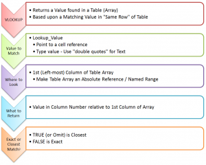
Each month, I get 5 to 6 emails of phone calls from viewers who who are having trouble using the VLOOKUP Function in Excel. In the majority of cases, the problem is that their Data Table is setup so that the “Key” field that they need to search in is NOT the Left-most or first field in the table. It is not always practical – nor desirable – to use “Cut and Paste” to rearrange the fields in the data set. So, what techniques can you use to fix this?

Use the OFFSET Function Inside a VLOOKUP Function

In this scenario, our IT Department sends us a daily report of the products that we sell including fields for the current cost and quantity on-hand. We use this report to generate additional reports and filters. This report gets saved automatically as an Excel 2010 Table with the name “Inventory.” The problem is, whenusing a VLOOKUP, that the first – or Left-most – field is NOT the “Key” field that we want VLOOKUP to use to search for a Match in order to return the current price or inventory for individual product.

The OFFSET() Function in Excel, makes it easy to reference a “starting field” that, in this case, is one column to the Right. This is perfect for our situation. We can continue to use our “named range” with the VLOOKUP!

Watch Video in High Definition

Follow this link to watch this tutorial in High Definition on my YouTube Channel – DannyRocksExcels

Visit My New Secure Online Shopping Website

I invite you to visit my new online shopping website at: http://shop.thecompanyrocks.com I have created new, extended length video tutorials that you can either purchase to download immediately or order them on a DVD-ROM. In addition, I have published versions of my 90 minute Pivot Tables Video Tutorials for Excel 2003, Excel 2007 and Excel 2010. So, I have the tutorials that you want for the Excel version that you are currently using!
Click to Play Excel Video Tutorial

Refer to an Excel Table Field When Writing Formulas

Refer to Excel Table in Formula

Refer to Excel Table in Formula

While I strongly recommend creating “Named Ranges” that you can refer to in an Excel Formula, there is one drawback. By default, “named ranges” refer to “Absolute” Cells – e.g. $A$1:$A$15

However, what happens when your data set expands? For example, when you add records beyond row 15 in this case.  Now, your formulas do not refer to the additional data in each field. You need to find a way to automatically expand the range of cells that your formula refers to.

Tables in Excel 2007 and Excel 2010

Fortunately, if you are using either Excel 2007 or Excel 2010, you can “format” your data set as an EXCEL TABLE and take advantage of many great options:

  • When you append records (rows) , the definition of your Table automatically expands.
  • You can “name” your table to reflect its contents. For example, in this video I name my Table – DRTable –  and I refer to it in my formulas.

Writing Formulas that Refer to Excel Table Field

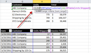
In this video tutorial I use the SUMIF Function. Remember that I have “named”my table DRTable. Here is how I begin my formula. =SUMIF(DRTable[Customer]. Notice the use of brackets ([ ]) around the [Customer] Field in the formula. This is the gotcha step in this lesson.

Watch This Video in High Definition on YouTube

I created this video tutorial in High Definition Mode. Click on this link to view it on my YouTube Channel – DannyRocksExcels

Get my best-selling DVD-ROM, “The 50 Best Tips for Excel 2007” – Visit my Online Bookstore for more information.

How to Trigger a Unique List of Values Based Upon Another Drop-Down List in Excel

You can use the INDIRECT() Function in Excel to create a drop-down list of unique values that is“triggered” by the label that you select in another drop-down list. In the scenario that I use in this lesson:

  1. Create your 1st Drop-down list using Data Validation in Excel – Allow “List.” Here the named range is “Departments.”
  2. Create a 2nd Drop-down list using Data Validation. This time the “list” uses the INDIRECT Function to reference the selected label from the 1st drop-down list.

Key Concept

 The labels in my 1st drop-down list serve as “named range” references. That is why the INDIRECT Function is able to pull up the correct list of “Job Titles” in the 2nd Drop-down list. For example, a reference to the text label “Sales” in the 1st drop-down list brings up a list of the values (Job Titles) from the “Named Range” (Sales) in the 2nd Drop-down list.

If you need to learn about – or review – Data Validation in Excel, follow this link to my free Excel video lesson on this topic.

Create Named Ranges in Excel

I have found that creating and using “Named Cell Range” references makes lookup functions and formulas so much easier in Excel. Watch this video to see how I use a variety of methods to Create Named Ranges in Excel. One tip is to use the Keyboard Shortcut “Ctrl + Shift + F3” – after you first select the Label and the Values for your Named Range.

In this lesson, I also demonstrate how to visually “flag” all of the cells that do not meet the criteria for your Data Validation. I find that most people are unaware that you can do this! I think that you will find many uses for this auditing tool as you work in Excel.

Additional Resources

Follow this link to watch this video on YouTube in High Definition, Full Screen Mode.

Here is the link to view the 2nd video in this series about the INDIRECT Function in Excel.

Learn how to “Master Excel in Minutes – Not Months!” – visit my new, secure shopping site – http://shop.thecompanyrocks.com

Two Ways to Produce an Executive Summary of an Excel List

On one of the technology blogs that I follow, there is a debate over the best way to produce an Executive Summary of the information in an Excel Data List. Some people like the idea of using Excel’s =SUMIF() Function for this while others recommend creating a Pivot Table as the summary.

You decide – after watching this short video demonstration using both approaches. And, add a comment or drop me an email to let me know your thoughts.

This Excel Video Lesson is available for you to download as a Podcast on iTunes.

Follow this link to go to the “Danny Rocks Tips and Timesavers” podcast.

Learn how to “Master Excel in Minutes – Not Months!”

How to Create Scenarios in Excel

Scenarios are part of Excel’s “What-If” Analysis tool set – aka Data Analysis. Use Scenarios when you need to know what the result will be when you change one or more variables in one or more  situations (scenarios).

Frequently, I create Scenarios to define  a “Good, Better, Best” or “Worst Case, Best Case, Case Most Likely” outcome.

In this short Excel Training Video, I demonstrate how to create, edit,  and report four Scenarios for a Monthly Office Expense Budget.

These are the steps used in this Excel Video Lesson:

  • Create (or open) an Excel worksheet that contains a formula. Identify the formula and the precedent  cells that feed into the formula.
  • Select the “target cell” – the cell that contains the formula whose result will change with each Scenario.
  • Choose TOOLS – SCENARIOS and follow the directions in the Create Scenario dialog box.
  • First, click ADD. Name the Scenario. Click OK. Confirm that you have selected the “Target Cell” and then click / type in the “Changing cells.” The Changing cells should be either direct or indirect precedents to the Target cell formula. Click Add. Add additional Scenarios as desired.
  • Click on the name of your Scenario and select SHOW to display the changing cell values and the new result in your target cell.
  • If you wish, choose SUMMARY to create a summary report in a separate worksheet.
  • I strongly recommend that you create named cells and use them in the formulas and changing cells of your Scenario.

NEW! Download the Excel Practice file used in this lesson:

Use my Index to search for the free Excel Training Video that you want to view.

New! Danny’s DVD Training Series, “The 50 Best Tips …” is now available at the online store for The Company Rocks

Related Videos