How to Combine 2 Excel Workbooks Using VLOOKUP Function

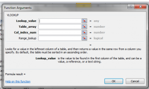
VLOOKUP Function Arguments

VLOOKUP Function Arguments

I created this video tutorial to assist one of my viewers. He had 2 Excel Workbooks that he needed to combine. Because he had a MemberID Field in each workbook, I decided that the VLOOKUP() Function would be the fastest way to complete this task for my viewer.

Tips Covered in this Video

  • Move or Copy a Worksheet to another Excel Workbook
  • Use a Mixed Cell Reference – e.g. $A4 – so that column “A” reference is “frozen” when copying formula
  • Create “Named Range” to use as the “Table_Array” argument in VLOOKUP
  • Use FALSE as 4th (optional) argument in VLOOKUP to produce an “exact match”
  • Use IFERROR to prevent “error messages” from displaying

Watch this Video in High Definition

Click on this link to watch this Excel Tutorial  in High Definition on my YouTube Channel – DannyRocksExcels

Learn About My Training Resources

I invite you to visit my secure online shopping website – http://shop.thecompanyrocks.com – to learn about the many training resources that I offer for sale.

Watch Tutorial Now



How to Search For and Use Text Strings in Excel

A viewer asked for my help in creating a report that will group his customers’ email addresses by their “domain name.” For example, he wants to be group all customers with gmail addresses . Likewise, his  customers’ yahoo mail, aol.com accounts, etc.

Pivot Table for Email Domains

Pivot Table Email Domains

I immediately decided to use two powerful Excel tools to produce this report:

  1. Text-to-Columns to create two columns (name and domain) from one text value (the email address).
  2. Pivot Table Report to group and present customer emails by domain name.

Both tools work great and I produced the report with only a few mouse clicks!

The response that I got from my viewer was, “That’s great Danny. But …”

It turns out that the viewer wanted to have the Domain Names as the Field Headers and to show each customer’s email address as a row going down vertically in the corresponding field. To give my viewer the report that he wanted, I used these tools and techniques:

  • I returned to the Pivot Table to copy the unique list of domain names.
  • I used Paste Special – Transpose to convert the vertical list of domain names into a horizontal row of Field Headers.
  • I began to build my “Mega-formula” by taking “baby steps” – i.e. I created one formula and then “nested” it inside additional formulas and functions.
  • For the first “baby step” formula I used the SEARCH() Function.
  • Next, I “nested” this formula as the “logical test” inside an IF() Function.
  • In order to “hide” all of the formula error signs, I nested both of these functions inside the NEW IFERROR() Function.
  • IFERROR() was introduced in Excel 2007 and I now consider it to be “indispensable!” This function, alone, makes upgrading to either Excel 2007 or Excel 2010 a “nobrainer” decision!

I enjoy answering questions from my viewers. Many of these questions can be answered from one of the lessons on my DVD-ROM, “The 50 Best Tips for Excel 2007.” For the rest, I try to create a video lesson that demonstrates how to get the answers that you – my viewers and customers – are looking for.

Keep your questions and suggestions coming! I enjoy receiving feedback from you!

I invite you to subscribe to my RSS Feed on Feedburner to be automatically notified whenever I publish a new Excel Video Tutorial.

Watch this Excel Video in High Definition on YouTube

Here is the link to watch this video on my YouTube Channel – DannyRocksExcels

When to Use Absolute, Relative & Mixed Cell References in Formulas

In my experience, I find that many Excel users get easily confused when it comes time to use an Absolute or a Mixed Cell Reference in a formula. Let me demonstrate how and when to use the proper cell references, so that you always get the correct result.

Here is what each type of cell reference looks like in a formula:

  • Relative Cell Reference – =A2*B2 when copied down one row becomes = A3*B3
  • Absolute Cell Reference – =A2*$B$2 when copied down one row becomes =A3*$B$2 (Notice the $B$2 Absolute cell reference in the formula)
  • Mixed Cell Reference – =$A2*B$3 when copied down one row becomes = $A3*B$3 and when copied one cell to the right becomes =$A*C$3 (Notice how one part of the cell reference is relative – it moves; and the other part of the reference is Absolute – it remains fixed in place)

Learn how to “Master Excel in Minutes – Not Months!”

Write a formula to total cumulative sales

Here are the steps to follow for this lesson:

  1. CHALLENGE: Write 1 formula in Column “C” to allow the range of values in Column “B” to expand by 1 cell each time the formula is copied down in Column “C.”
  2. In cell C2, the formula is =SUM(B$2:B2)
  3. Notice the $ in the cell reference on the left side of the range = SUM(B$2…
  4. The $ creates a “Mixed Cell” reference in the formula. This allows the range of cells in our formula to expand when we copy the formula down in Column “C.”
  5. Learn how to clear the “Green Triangle” Smart Tags in a range of cells.

Find the video lesson that you want – Index to all Excel Topics

News! My DVD, “The 50 Best Tips for Excel 2007” is now available to purchase. I invite you to visit my online bookstore for more details.