How to Correct #N/A Error Messages for Excel’s VLOOKUP Function

Fix the #N/A Error Message

A colleague of mine – who is an experienced Excel user – cannot figure out why he is receiving those ugly #N/A Error Messages when he is using the VLOOKUP Function in Excel.

After a quick look at his workbook, I spotted the problem!

Use the TRIM() Function to Remove Extra Spaces

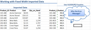
It turns out, that the data source – housed on the company’s Main Frame Computer – is using “Fixed Width” Fields. So, while only 7 characters are visible, I used the LEN() Function to determine that the field was actually storing 12 characters.

The #N/A Error Message for VLOOKUP()

The #N/A Error Message appears when a Match cannot be found for the Lookup Value in the Left-most Column of the Table_Array when using VLOOKUP(). In this case, my viewer was trying to match a lookup value that contains 7 characters to a value in a field formatted to contain 12 characters. This is what produced the #N/A Error!

Paste Special Values

The final step to correct this problem is to use Copy – Paste Special – Values to replace the Formulas with the values of those formulas.

Essential Excel Skills

9 Essential Skills for Excel 2010

9 Essential Skills for Excel 2010 Video Tutorial

In this video, I cover three Essential Excel Skills:

  1. Essential Functions – VLOOKUP()
  2. Text Functions – LEN() and TRIM()
  3. Paste Special Options

I cover each of these skills – and more – in greater detail on my new 4-Hour Video Training Resource, “Nine Essential Skills for Excel.”” Click on the links below to learn more about:

Watch Video in High Definition

Follow this link to watch my Excel tutorial in High Definition on my YouTube Channel – DannyRocksExcels

How to Combine 2 Excel Workbooks Using VLOOKUP Function

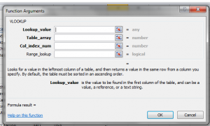
VLOOKUP Function Arguments

VLOOKUP Function Arguments

I created this video tutorial to assist one of my viewers. He had 2 Excel Workbooks that he needed to combine. Because he had a MemberID Field in each workbook, I decided that the VLOOKUP() Function would be the fastest way to complete this task for my viewer.

Tips Covered in this Video

  • Move or Copy a Worksheet to another Excel Workbook
  • Use a Mixed Cell Reference – e.g. $A4 – so that column “A” reference is “frozen” when copying formula
  • Create “Named Range” to use as the “Table_Array” argument in VLOOKUP
  • Use FALSE as 4th (optional) argument in VLOOKUP to produce an “exact match”
  • Use IFERROR to prevent “error messages” from displaying

Watch this Video in High Definition

Click on this link to watch this Excel Tutorial  in High Definition on my YouTube Channel – DannyRocksExcels

Learn About My Training Resources

I invite you to visit my secure online shopping website – http://shop.thecompanyrocks.com – to learn about the many training resources that I offer for sale.

Watch Tutorial Now


Working With Array Formulas in Excel

There are at least two benefits to using an Array Formula in Excel:

  1. They will speed up creating your formulas by, in many cases, eliminating intermediate formulas.
  2. They will add a level of protection to your formulas because you cannot edit the individual cells in an Array Formula. You must edit “all” of the cells.
Array Formulas
Array Formulas

In this lesson, I first demonstrate how to select and use arrays with the SUMPRODUCT() Function in Excel. SUMPRODUCT is a very handy function to use when you want to first multiply (PRODUCT) the cells in two or more arrays and then total (SUM) the results.

 
Next, I demonstrate two ways to create Array Formulas. Notice that in the second example that it is important that you remember to select ALL of the cells that will contain the results of the Array Formula. It is vital that all arrays are of Equal Size (Same number of cells in the same dimension – horizontal and vertical).
 

Entering Array Formulas

Use the keyboard combination of Ctrl + Shift + Enter when entering an Array Formula. Do not press the Enter key alone – this will result in an Error for your formula! Some people refer to Array Formulas as CSE Formulas to remember the Ctrl + Shift + Enter combination. Notice, in the Formula Bar,  that Excel automatically adds { braces } around the Array Formula. Do not enter these manually.

Editing Array Formulas

You gain a level of protection for your formulas when you use Array Formulas because you cannot select a single formula cell to edit it. You must select all of the cells that contain the Array Formula before you can edit it – or delete it. If you don’t select all of the cells first, you receive an Error message in a pop-up window. Remember to press the “CSE keyboard combination” when you complete your edit of the Array Formula.

Learning to use Array Formulas is an essential skill to acquire if you want to master Excel. I guarantee that you will be able to write more accurate formulas when you use arrays.

Watch this Video on YouTube

Click this link to watch this Excel Video in High Definition, Full Screen Mode on my YouTube Channel – DannyRocksExcels

Learn how to “Master Excel in Minutes – Not Months!”

Use Excel’s Goal Seek to Find Formula Error

A viewer wrote me seeking help with a formula. He was calculating a monthly payment for a loan using Excel’s PMT() Function and he was surprised at the result of the formula. I reviewed his formula and discovered that it was not a “formula problem.” Rather, it was a “results problem!” Watch this short video to see how I solved this problem for my viewer by using Excel’s “Goal Seek” tool. So now, instead of a monthly payment of $10,666.67, the result is $501.38 – a very different result!

You can download this video – for free – here on my website. Just click the button below the video image.

You can also subscribe to my Podcast, “Danny Rocks Tips and Timesavers” at the iTunes Store.

You can “Master Excel in Minutes – Not Months!”