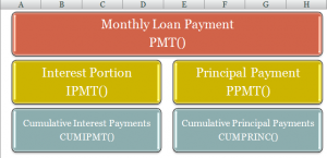
When you use the PMT Function in Excel, the result is the amount of money that you will pay each period (usually monthly) until the loan is repaid. When you want to know how much of each payment is an interest charge, you use the IPMT Function. And,to find the amount that goes towards reducing the principal on your loan, you use the PPMT Function.
Cumulative Payments
Two other functions are helpful in analyzing your loan payments. When you want to see the Cumulative amount of Interest (CUMIPMT Function) that you paid between two periods – e.g. Starting with payment 1 and ending with payment 12. You use the CUMPRINC Function to total the amount of your loan payments that went towards reducing the principal on your loan between any two periods.
Absolute and Relative Cell References
As you will see in the video, I use a combination of Absolute Cell References (e.g. $A$4) and Relative Cell References (e.g. A4) in these formulas. An Absolute Cell Reference means that cell will “remain in place” when the formula is copied down or across to other cells. In this example, I have my Loan Information (Amount to borrow, Interest Rate, etc.) at the top of the spreadsheet. Almost all references to these cells in formulas is Absolute.
Function Arguments Dialog Box
I almost always use the Function Arguments Dialog Box when I am creating my formulas. I use the Keyboard Shortcut, Ctrl + A at this point in the formula – “=PMT(” to activate the dialog box. The advantages of using the Function Arguments Dialog Box are:
- Explanation of both the function and each “argument” in the function
- Ensures arguments are answered in the proper sequence
- Ensures that all “required” arguments (Argument Labels are in Bold)
- Evaluates the result of each “intermediate” calculation – to the right of each argument
This is the first of several Excel Video Lessons that I am creating to demonstrate how to perform Financial Calculations. Let me know what you think or send me your questions to answer. You can add a comment below this post.
Watch This Video in High Definition on YouTube
Follow this link you view this Excel Video on my YouTube Channel – DannyRocksExcels
Download Excel Workbook
Follow this link to download the Excel Workbook I used in this lesson.
Subscribe to My Video Podcast
I invite you to receive an automatic notice – via email – whenever I publish a new Excel Video Lesson. Follow this link to find out the details. The subscription is free; you do not need to provide and personal information beyond your email address; and you can cancel at any time – no questions asked!


