Summarizing Employee Hours Worked and Vacation Time over 52 Weeks in Excel

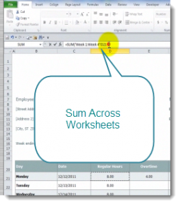
Sum Across Worksheets

Sum Across Worksheets

This is the third episode in my series of Excel Tutorials where I share my best practices for creating an Excel Workbook that contains 52 weeks of Employee Time Cards. In this lesson, I focus on techniques to Summarize – or Consolidate – the hours worked or taken as vacation, by each employee, over a period of several weeks.

Sum Across Worksheets

This is a great tip to learn! In my experience, I find that very few experienced users of Excel know that you can do this! This will eliminate the hassle of linking to a cell in individual worksheets to create your formula. There is, after all, a limit to the number of characters that you are allowed in a formula!

Consolidate Data By Position

Since each worksheet in this workbook is identical in structure, Data Consolidation is simple. Provided, that is, that you remember to “Add” each worksheet range reference in the Dialog Box. In this example, I have “created a link” to each worksheet so that the data can be easily updated.

Links to Other Tutorials in this Series

Shop for Additional Resources

I invite you to visit my new, secure online shopping website – http://shop.thecompanyrocks.com – where you can preview all of the resources that I offer you.

Watch Tutorial in High Definition

Follow this link to view this Excel Tutorial in High Definition on my YouTube Channel – DannyRocksExcels

Use an Excel Template to Customize a Worksheet with 52 Weeks of Employee Time Cards

Template for Time Cards in Excel

Time Card Templates in Excel

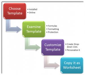
This is Part Two in my new series of Excel Tutorials where I share my best practice tips for creating 52 weeks of Employee Time Cards – for hours worked. In this segment, I focus on starting the process with an Excel Template.

Finding Templates for Time Cards

As I demonstrate in the video, there are at least two easy sources for finding a Time Card Template:

  1. Sample Templates Installed on your Computer
  2. Templates that you can preview and download from the Microsoft Office Templates Website

Examining Templates that You Download

Before you even think about duplicating the Excel Template that you just downloaded, it is important for you to take a few minutes to explore:

  • The Formulas used in the Template
  • The Formatting used in the Template – especially the formatting for Dates and Times
  • The Protection Applied (if any) to the cells or the entire worksheet

Creating Drop-down Menus for your Template

Since our premise here is that we will copy the template to 51 additional worksheets, it makes sense to use Data Validation to create a series of “drop-down menus” for Employee names and the Start Date for each week. I demonstrate how to do this in the video tutorial.

Links to Additional Video Tutorials in this Series

Additional Resources for Excel

I invite you to visit my new, secure, online shopping website – http://shop.thecompanyrocks.com – to discover the many training resources that I offer you!

Watch Tutorial in High Definition

Follow this link to watch this Excel Tutorial in High Definition on my YouTube Channel – DannyRocksExcels

Click to Watch Video Now

Dynamically Update a Cell with an Excel Worksheet Name

Formula to Capture Worksheet Name

Capture Tab Name in Cell

I am excited to share this Excel Tip with you! Several viewers have recently asked if there was a way to create a link in a cell to the name of a worksheet tab. Yes there is! And, in this lesson, I demonstrate how to do this.

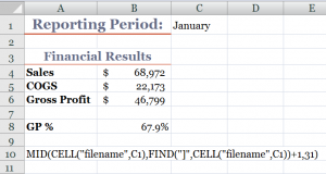
Say, for example, that you want Cell C1 to contain the name of the current worksheet (Sheet1). With this formula, when you change the name of the worksheet to “January,” cell C1 is dynamically updated to show “January.”

Perfect for Excel Templates

If you use a template for your monthly, regional sales or financial reports, then this Excel formula is essential. You write the formula once – using Group edit – and each worksheet in your Excel workbook will be linked to a cell in your report. Change the name of the worksheet and your report name is automatically updated.

Functions Used in this Formula

  • CELL() – to gather information about the worksheet – in this case, the “Filename.”
  • MID() – to extract the characters in a text string – e,g, the “worksheet name.”
  • FIND() – to locate the starting point for the MID() function to extract the characters in the text.

As the final argument for the MID() Function, I use 31 characters because that is the maximum number of characters that you can use when naming an Excel worksheet.

Try this for yourself. Let me know how it works for you. Add your comments below.

Download Excel Workbook for this Lesson

Watch Video in High Definition

Follow this link to view this video tutorial on my YouTube Channel – DannyRocksExcels

I invite you to watch or to subscribe to my video podcast on iTunes. Follow this link to learn more about my RSS Feed.

Consolidate Excel data by position

Most companies use Excel to produce budget reports. In this video lesson you will learn how to consolidate data from January, February and March to produce a 1st Quarter Consolidated Budget report – based off of an Excel Template.

Here are the steps to follow in this video lesson:

  1. Start with a Template – either on your computer or download one from the Microsoft website. Modify as necessary and then make multiple copies of it. e.g. 1 ea. for Jan, Feb, Mar and 1st Qtr, etc.
  2. Select the 1st cell to receive consolidated data in your 1st Quarter Consolidated report. Then, choose Data, Consolidate.
  3. Point to the January worksheet and select the range of cells that you want in the 1st Qtr consolidated report. Then click ADD.
  4. Repeat this process pointing to the February and March worksheets. Because we based our monthly reports on a Template, the range of cells in each worksheet is exactly the same – i.e. “By Position.”
  5. If you do not check the “Create links to source data” box, you will simply add (SUM) the data from the selected ranges into the Consolidation worksheet. SUM is the most common function but you are free to choose others.
  6. If you did check the “Create links to source data” box your consolidation worksheet will be outlined and each cell will be linked back to its source cell.

Find the Excel Video Lesson that you want – Index to all Excel Topics

News! My DVD, “The 50 Best Tips for Excel 2007” is now available to purchase. I invite you to visit my online bookstore for more details.

Related Excel Video Lessons