Structured Formula References in Excel 2007 and Excel 2010 – Part 2

Compare Structered References Excel 2007 v 2010

Compare Structured References 2007 v 2010

This is the second and concluding part of this series where I demonstrate how to use Structured Formula References when referring to Excel Tables.

Key Points Covered

  • The difference between Structured Formula References in Excel 2007 and Excel 2010
  • How to Edit Structured Formula References
  • How to Write Structured Formulas using the new Formula AutoComplete drop-down menu


Watch My Video Tutorial Now


Watch Video in High Definition on YouTube

Click on this link to watch this Video in High Definition on my YouTube Channel – DannyRocksExcels

Go to Part 1 in this Series of Video Tutorials

Follow this link to go to Part 1 in this Series of Tutorials about using Structured Formula References in Excel Tables.

Visit My New Secure Online Store

I have just published 6 New Products and opened a new, revised, secure online shopping website. Take a look at: http://shop.thecompanyrocks.com
 

How to Use Structured Formula References for Tables in Excel 2007 and Excel 2010

Structured Formula Reference - Excel 2007

Structured Formula Reference - Excel 2007

Beginning with Excel 2007, you can – and should – convert a Standard Data Range to an Excel Table. Doing so offers several advantages:

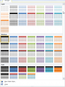
  • You get a selection of Table Styles – including Alternate Row Shading – that make it easier to read your tables.
  • You can automatically extend the Scope of your Table – by adding additional Fields (Columns) or Records (Rows).
  • You can give your Table a “Name” to reflect the purpose of the Table.
  • You can add a Total Row to Subtotal each Field (Column) and you can change the Function used to Subtotal from a drop-down menu.
  • You can apply Structured Formula References in the Table – Enter the Formula in a Single Cell and it is Automatically copied down for each record in the Table.

“In This Row” Formula Styles

Structured Formula References use a new style of formulas. Rather than referring to a specific Cell, in an Excel Table, you refer to a Field “in this row.” This type of formula is easy to create “inside the table.” It is also fairly easy to create “outside the Table” using the new Formula AutoComplete tool. You will be using [ ] (Left & Right Brackets) for these formulas. I go over these details, in-depth, in this video tutorial.

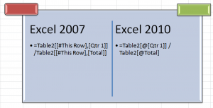
There are also distinct differences in how Structured Formula References are created between Excel 2007 and Excel 2010. These Structured Formula References are greatly streamlined in Excel 2010 – in my opinion.

The SUBTOTAL() Function and Excel Tables

I strongly recommend that you become familiar with how to use the valuable SUBTOTAL() Function in Excel when referring to the data in a Table. With the SUBTOTAL Function, you can produce a wide range of summaries anywhere on your Excel Workbook. And… the Subtotal Results reflect the totals for any “Filters” that you apply to your Table.

Play this Video in High Definition

Watch this Video in High Definition

Follow this link to watch this Excel Tutorial in High Definition on my YouTube Channel – DannyRocksExcels

Go to Part 2 in this Series of Tutorials

Follow this link to go to Part 2 in this series of tutorials about using Structured Formula References in Excel Tables.

Announcing 6 New Products on My New Online Secure Shopping Website

I invite you to visit my new online shopping site. I have added 6 new products – Extended Length Video tutorials that you can either “download now” or purchase as a DVD-ROM. Each product contains over 90 minutes of in-depth video instruction for Pivot Tables. You can choose the product to fit your version of Excel – Separate products for Excel 2003, Excel 2007 and Excel 2010.

Click here to view my new products.

How to Create a Summary Report from an Excel Table

Functions for Executive Summary

Functions for Executive Summary

I created this Excel Video Tutorial in response to a viewer who, in her company, is not permitted to use a Pivot Table to create a report. Unfortunately, this happens more often than you might think. Nevertheless, I promised to share my tips and advice. I think that many of this tips will help Excel users at all levels.

Tips Covered in this Video Tutorial

  • Use Advanced Filter to Extract a list of unique customer names from a range with @ 4,300 records.
  • Later in the lesson, I show you how to extract this list to a different worksheet – a tip that will save you time when preparing your reports!
  • How and why to convert a normal range of data into a TABLE in Excel 2007 / 2010 or into a LIST in Excel 2003.
  • How to create “Named Ranges” for your key data cells and to use them in your Formulas and Functions.
  • How to use the SUMIF, AVERAGEIF and COUNTIF Functions in your summary report.

Keyboard Shortcuts Used in this Tutorial

  • Ctrl + T to convert to a TABLE in Excel 2007 / Excel 2010
  • Ctrl + L to convert to a LIST in EXCEL 2003
  • Ctrl + A to open up the Function Arguments Dialog Box
  • Ctrl + Shift + F3 to open the Create Names Dialog Box
  • F3 to open the Paste Names Dialog Box

I decided that I will only make this video available on YouTube – I think that you will enjoy the clarity that you get from the High-Definition / Full Screen Mode.

Watch Tutorial in High Definition on YouTube

Follow this link to view this Excel Tutorial in High Definition on my YouTubeChannel – DannyRocksExcels

Visit my new secure online shopping website

I invite you to visit http://shop.thecompanyrocks.com – my new online shopping website.

Watch Video Now

How to Take Advantage of Excel 2007 – 2010 Tables and Excel 2003 Lists

Excel Table Styles

Excel Table Styles

In this video tutorial, I cover multiple versions of Excel. I demonstrate how to take advantage of the Table Tools that were introduced in Excel 2007 and I also show you how to create Excel 2003 Lists.

Topics Covered on Video Tutorial

  • Convert a range of data to an Excel 2007, Excel 2010 Table.
  • Convert a range of data to an Excel 2003 List.
  • View and change the Total Row in each version of Excel.
  • Append new records to Tables and Lists.
  • Add a new field to Tables and Lists.
  • Write a formula in one cell of an Excel Table and have it automatically copy down for each record.
  • Change the Table Styles in Excel 2007 and 2010.
  • Use Conditional Formatting to add alternate row shading to an Excel 2003 List

Watch Video in High Definition on YouTube

Follow this link to watch this Excel Video Tutorial in High Definition on my YouTube Channel, DannyRocksExcels

Download This Excel Workbook

Click on this link to download the Excel Workbook that I used in this video tutorial.

Get my best-selling DVD-ROM, “The 50 Best Tips for Excel 2007” for only $39.95!

Refer to an Excel Table Field When Writing Formulas

Refer to Excel Table in Formula

Refer to Excel Table in Formula

While I strongly recommend creating “Named Ranges” that you can refer to in an Excel Formula, there is one drawback. By default, “named ranges” refer to “Absolute” Cells – e.g. $A$1:$A$15

However, what happens when your data set expands? For example, when you add records beyond row 15 in this case.  Now, your formulas do not refer to the additional data in each field. You need to find a way to automatically expand the range of cells that your formula refers to.

Tables in Excel 2007 and Excel 2010

Fortunately, if you are using either Excel 2007 or Excel 2010, you can “format” your data set as an EXCEL TABLE and take advantage of many great options:

  • When you append records (rows) , the definition of your Table automatically expands.
  • You can “name” your table to reflect its contents. For example, in this video I name my Table – DRTable –  and I refer to it in my formulas.

Writing Formulas that Refer to Excel Table Field

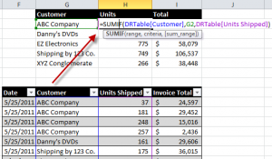
In this video tutorial I use the SUMIF Function. Remember that I have “named”my table DRTable. Here is how I begin my formula. =SUMIF(DRTable[Customer]. Notice the use of brackets ([ ]) around the [Customer] Field in the formula. This is the gotcha step in this lesson.

Watch This Video in High Definition on YouTube

I created this video tutorial in High Definition Mode. Click on this link to view it on my YouTube Channel – DannyRocksExcels

Get my best-selling DVD-ROM, “The 50 Best Tips for Excel 2007” – Visit my Online Bookstore for more information.