Use Excel’s AutoFill Options and Formulas to Increment a Series of Dates

Excel AutoFill Options

Excel AutoFill Options

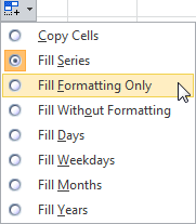
I begin this Excel Video tutorial by first, demonstrating how to use Excel’s AutoFill Options to increment a series of dates. Some of these AutoFill Options are:

  • Fill Weekdays Only (Monday through Friday)
  • Copy Formatting Only
  • Increment by Adding one month to the previous cell
  • Increment by Adding one year to the previous cell

Here’s a Tip: If you use your Right-mouse button to AutoFill a series, a menu of options will pop up automatically when you release the mouse. Try it!

Excel Functions and Formulas to Increment a Series of Dates

Two of my favorite Excel Date Functions are part of the “Analysis ToolPak” Add-in:

  1. The EDATE() Function – returns a “serial number” for a Month that is X number of months away from the starting date.
  2. The EOMONTH() Function – is similar to EDATE. However, it always returns the last Calendar Day of the Month that is X  number of months away from the starting date.

In Excel 2007 and Excel 2010, the Analysis ToolPak Add-in is activated by default. In this video, I demonstrate how to activate it if you are using Excel 2003 or older.

Other Functions Used in this Video Tutorial

  1. The DATE() Function. Remember that if you use this function to increment by one-year intervals that you need to “nest” the Year(), Month() and Day() functions in the arguments. This is a “tricky” function to use.
  2. The WEEKDAY() Function. In the video, I nest this function inside an IF() Function in order to get a series of dates that include Monday through Friday only!

Related Video Tutorial

My next video in this series demonstrates how to use Formulas to increment a series of times by “minutes” or by “hours.”

Watch This Video in High Definition

Follow this link to view this video tutorial in High Definition on my YouTube Channel – DannyRocksExcels

Shop for Excel Training Resources

Shop for The 50 Best Tips for Excel 2007

Shop for The 50 Best Tips for Excel 2007

I invite you to visit my secure online shopping website – http://shop.thecompanyrocks.com – to see all of the great training resources that I offer you.

Get my best-selling DVD-ROM, “The 50 Best Tips for Excel 2007” for only $39.95!


How to Use Date Functions and Date Formatting in Excel

In this lesson, I respond to two recent requests from viewers for help in Using DATE Functions in Excel and also, how to apply Custom Date Formatting. I get similar requests on a frequent basis from both viewers and clients.

Solve Problem #1 

My first viewer wants help in using the DATE() Function in Excel. She wants to calculate a date that is 90 days after the starting date for a project. She encountered two problems

  1. Initially, the DATE() Function produced and error – because she forgot to ‘nest” the YEAR(), MONTH()+9, DAY() Functions inside the DATE() Function.
  2. She was not expecting a date to be filled in the formulas column when there was no starting date for the project – She needed to include an IF() function to perform a LOGICAL TEST – Does  the Starting Date = 0, Value if TURE, ” ” (to display nothing), Value if FALSE – to perform the calculation.
Excel Custom Date Formats

Excel Custom Date Formats

Solve Problem #2

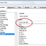
My second viewer wanted my help to ensure that the date values that he “pasted” into a range of cells were in the (Custom) format of “yyyy-mm-dd” (Year, Month, Date).

In this case, we need to take two steps:

  1. Format the destination cells using the CUSTOM FORMAT of yyyy-mm-dd that we create.
  2. After “Pasting” the Copied Cells, use the “Paste Options” dialog box to select – “Match Destination Formatting.”

I also demonstrate how to use the NETWORKDAYS() Function and the WORKDAY() Function – with an optional list of “Holidays” to exclude. And, finally, I show you the “pitfalls” that occur when you import a “text” file of dates that use a variety of formats. In order to perform DATE calculations, a date must be stored as a NUMBER in Excel. It must be right-aligned in the cell.

You can watch this Excel Video Lesson in High Definition, Full Screen Mode on my YouTube Channel – DannyRocksExcel – by clicking this link.

Learn to “Master Excel in Minutes – Not Months!”

Learn How to Use Date Functions in Excel

Excel has a group of functions that help you to calculate dates. For example, the number of days between two dates or the date on which an invoice will be payable.

This is the second in my series of lessons where I demonstrate how to enter and calculate dates and times in Excel. Here is the link to part one.

Excel Tip List

Excel DVD Tips

The date functions that I demonstrate on this video are:

  • TODAY()
  • NOW()
  • DATE()
  • DATEVALUE()
  • WORKDAY()
  • NETWORKDAYS()
  • EOMONTH()

The last three date functions require you to activate the Analysis ToolPak Add-in. You will also learn some valuable and time saving keyboard shortcuts.

You can watch this video in High Definition, Full Screen Mode on my YouTube Channel – DannyRocksExcels

Learn how to “Master Excel in Minutes – Not Months!”

Use the =SUMIF() Function to Tally YTD Sales

Many of my clients keep a “running total” of sales. They put “Dates” in Column “A” and enter each day’s sales in Column “B.” Next is Column “C” which contains the formula =SUM(B$:B250). That is fine – it works.

However, if you use the =SUMIF() function to total Year-to-Date (YTD) Sales you gain flexibility, save space and save time – because you do not have to scroll down several screens to see your YTD Sales total!

In this video, I show you how to use “Named Ranges” in a =SUMIF() Formula to keep track of your cumulative sales total.

Here are the steps to follow in this lesson:

  1. Traditionally, you use a formula like =SUM(B$3:B250) to give you a “running total” for YTD Sales.
  2. The=SUMIF() Function returns the SUM of vales that meet a “Single Criterion” (the IF portion) .
  3. The 1st Argument is – What is the Range that you want your criteria to evaluate? Consider “Naming” this Range – it makes it easier to write your formula and explain your formula.
  4. The 2nd Argument is – What is your criteria? Be sure to use this syntax – “Comparison Operator”
  5. In the video example we also need to include the “&” to join the cell “D2.” Cell “D2,” in this example, contains the Function =TODAY()
  6. The 3rd Argument is – What Range do you want to SUM to return the values that meet your Criteria?
  7. The =DATE() Function returns the serial number for a specific date. It requires 3 Arguments. =Date, Year, Month, Day)
  8. You will save time and gain productivity when you “Name Cells and Ranges” and then you them in your formulas.
  9. Use the F3 shortcut key to “Paste Names” into your formulas.

News! My DVD, “The 50 Best Tips for Excel 2007” is now available to purchase. I invite you to visit my online bookstore for more details.

Find the Excel Video Lesson that you want – Index to all Excel Topics