How to Use Multiple Sorting Options in Excel

Sort Using Cell Icons

Sort based on Cell icons in Excel

Beginning with Excel 2007, the Sorting Commands gained several new features and became much more powerful. For example, you are no longer limited to three levels of sorting. You can sort using as many levels as you need. In addition, you can now sort by Cell or Font Colors and also sort using the new Cell Icons.

While I was training one of my clients last week, several questions about sorting came up. So, in this video I will demonstrate several of the new features as well as showing you how to take advantage of many sorting options that have been around for some time. For example, using a Horizontal Sort to quickly rearrange the order of your columns!

Sorting Options on Video Tutorial

Here are the sorting options that I demonstrate on my video:

  • Sort on Values using a Custom List
    • First, I use a built-in custom list (Months of the Year).
    • Next, I demonstrate how to create a custom list that you can use with AutoFill and also with custom sorting.
  •  Sort data based upon Cell Icon
    • Cell Icons were introduced in Excel 2007 as part of the major upgrade to Conditional Formatting.
  • Sort Horizontally to quickly rearrange the order of your columns (fields) in your data set.
    • This feature has been available for many years. However, in my experience, very few people are aware of its existence.
    • Once you  learn this technique, you can stop the tedious task process of Insert Column, Cut Column, Paste Column, Delete Column, etc.

Shop for Excel Training Resources

I invite you to visit my secure online shopping website – http://shop.thecompanyrocks.com –   where I offer a range of video training resources for all of the Microsoft Office Programs.

Watch My Video in High Definition

Follow this link to watch my video in High Definition on my YouTube Channel – DannyRocksExcels

How to AutoFill the Letters in the Alphabet in Excel

 One of my viewers would like to be able to AutoFill the Letters in the Alphabet in his Excel Workbooks – he creates Alpha-Numeric Part Numbers for his products.

Two Ways to AutoFill Letters in the Alphabet

  1. Use a Formula – =CHAR(ROW(A65)) and AutoFill Down in the Column – This is not ideal
  2. Create and Use a Custom List in Excel. – So, use the Formula to create your list of 26 Alphabetical Letters. Copy the List and use Paste Special Values to convert the formulas to values. Then create your Custom List.

Using the CHAR() Function in Excel

There are 255 ASCI Characters that you can use in Formulas. For example, =CHAR(169) will return the © Symbol. In this lesson, I share a great Keyboard Shortcut that you can use to add this Symbol into the Footer of your printed Excel worksheet – Watch the video to discover this!

Visit My Secure Online Shopping Site

I hope that you take a few minutes to visit my new, secure online shopping website. The address is: http://shop.thecompanyrocks.com


Watch Tutorial in High Definition

On my YouTube Channel – DannyRocksExcels – I have posted this tutorial in High Definition Mode. Click here to go directly to this video.
 

Working with Custom Lists in All Versions of Excel

Edit Custom Lists in Excel

Edit Custom Lists in Excel

Custom Lists in Excel are great because the help to ensure accuracy and consistency when entering data on a worksheet. Excel comes with several Custom Lists built-in to the program – e.g. Days of the Week and Months of the Year. Now, you can quickly use Excel’s AutoFill handle to add Jan, Feb, Mar, Apr, etc. in any direction (vertical or horizontal) on the active worksheet.

Edit Custom Lists

You can quickly create – or edit – your own Custom List. Follow these steps:

  1. Type your list in a contiguous group of cells – either vertically or horizontally.
  2. Select the cells with the values that you just entered.
  3. Spell check this list – use the F7 Keyboard Shortcut
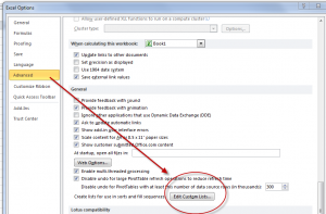
  4. Open up the Edit Custom List Dialog Box. (Watch this video to see how this is differs between Excel 2010, Excel 2007 and Excel 2003.)
  5. With your new Custom List selected, click the “Import” button to add your Custom List to the current version of Excel on this computer.

Sort Data Using a Custom List

On this video tutorial, I demonstrate how to sort a list of data using a Custom List – e.g. to get the “Month” field sorted in chronological order (January, February, etc.) This will save you a great deal of time!

Create a Custom List for Letters of Alphabet

Having a Custom List for the 26 letters of the alphabet comes in handy on many occasions. I show you how to AutoFill down the initial list using =Char(Row() + 64) beginning in Row 1 – a really usefuly function!

View This Excel Video Tutorial in High Definition

Follow this link to watch this video tutorial in High Definition on my YouTube Channel – DannyRocksExcels

Get my best-selling DVD-ROM, “The 50 Best Tips for Excel 2007” for only $29.97!

How to Sort Using a Custom List in Excel

What happens when you sort a list of Months in the Year in Ascending Order? You will get “April, August …, etc.” And that, I guarantee, is not what you want! So, how do you get the list to sort as “Jan, Feb, Mar, … etc.?

Sort Using a Custom List

Sort on Custom List

Sort on Custom List

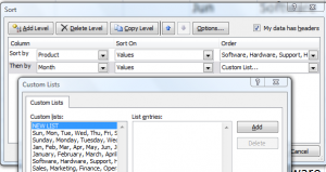
The months of the year and the days of the week are Custom Lists that are built into Excel by default. You can also create your own Custom Lists – e.g. a list of department in the order that you want to see them displayed. Once you have a Custom List saved in Excel, you can choose to sort using this order.

Watch this short video lesson to see how to create a Custom List and also how to Sort Using a Custom List in Excel.

High Definition, Full Screen Mode on YouTube

Here is the link to watch this video on my YouTube Channel – DannyRocksExcels
Learn More About Custom Lists in Excel

I have identified “Creating Custom Lists to AutoFill and Sort By” as an Essential Skill in Excel. I have created a four-hour comprehensive video training package that covers the “Nine Essential Skills in Excel.”  Click on these links to learn more about my video training resources:

Create a Custom List to AutoFill

Custom lists in Excel do two things very well:

  1. They speed-up your data entry
  2. They ensure accurate data entry

In this video lesson, I demonstrate how easy it is to create and employ Custom Lists in Excel.

Here are the Steps to Create a Custom List in Excel:

  1. Type the values for your list in either a column or a row
  2. Select the list of values and Spell Check them (F7)
  3. From the TOOLS Menu select OPTIONS and the CUSTOM LIST in the Dialog Box
  4. Since we already have selected the list of values click IMPORT

You can now use your custom list for data entry in ANY worksheet and ANY workbook on your computer.

NEW! Download the Excel practice file I use in this lesson: create-custom-lists

Find the video lesson that you want – Index to all Excel Topics

News! My DVD, “The 50 Best Tips for Excel 2007” is now available to purchase. I invite you to visit my online bookstore for more details.

Related Videos

Related Excel Videos