How to Calculate the Calendar Year Quarter for a Date in Excel

Formulas to Calculate a Calendar Year Quarter

Formulas to Calculate a Calendar Year Quarter

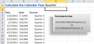
After watching my previous video tutorial, “How to Place Dates in a Fiscal Year Quarter,” several viewers requested that I demonstrate how to calculate the calendar year quarter for a date.

This requires “nesting” the MONTH() /3 Function inside either the ROUNDUP() or the CEILING() Function. I break these formulas down step-by-step in this video so that you can see how they work.

Formatting Numbers to Include Text

As a bonus, I demonstrate how to format the formula result cells to include the text “Quarter.” This is really simple to create as a custom format.

Download this Video Podcast from iTunes

You can watch and download this – and many of my – video tutorials for free at iTunes. Here is the link to my iTunes video podcast, “Danny Rocks Tips and Timesavers.”

Watch Video in High Definition

Follow this link to watch this Excel Tutorial in High Definition on my YouTube Channel – DannyRocksExcels

Visit my Secure Online Shopping Website

I invite you to visit my online shopping site – http://shop.thecompanyrocks.com – to preview and purchase my training resources. I guarantee your satisfaction 100%. I will refund your purchase if, for any reason, you are not satisfied with my products!


Formatting an Excel Pivot Table Frequency Report

Show % in Frequency Report

Show % of in Frequency Report

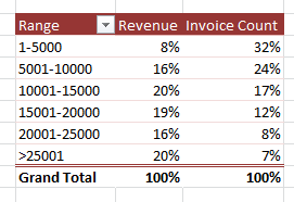
This is Part 2 of my 2-part series on Excel Pivot Table Frequency Reports. A Frequency Report is a great way to answer these questions:

  • How many invoices did we generate for values under $5,000?
  • How many invoices did we gererate for values over $15,000?

In this part, I show you how to format the Frequency Report to make it easier to present the information.

Formatting the Frequency Report

Here are the changes that I made to improve the look of the Frequency Report:

  • Reduced the number of “bins” in the frequency range by changing the “Grouping.”
  • Changed the formatting to make large numbers (millions) easier to read – e.g. as $3.2M
  • Made a copy of the Pivot Table to show values as “% of Total.”

Click on this link to go to Part 1 in this series of video tutorials for Pivot Table Frequency Reports

Learn How to Use Pivot Tables

I have created a series of video tutorials that you can download to learn how to create and modify Excel Pivot Tables. You can choose to download the recording that fits your version of Excel (2003, 2007 or Excel 2010). The cost is $9.95 for the video recording and that includes the Excel workbooks that I used and a step-by-step instructional manual. Follow this link to get more information about these recordings.

Watch this Video in High Definition on YouTube

Follow this link to watch this video tutorial on my YouTube Channel – DannyRocksExcels

Make it Easier to Display Large Numbers in Excel with Formatting Codes

In order to establish and maintain your credibility, the numbers that you store in Excel must be accurate and precise. You cannot compromise on this principle! In most cases, you will be working with large numbers – sometimes, very large numbers. And, this may present a problem when you need to present these numbers to your audience.

So …

It is essential that you distinguish between your need to maintain accurate “data” and your need to communicate the essential “information” that resides in your data to your audience.

Format Custom Numbers

Format Custom Numbers in Excel

When you are presenting the “essential information” that resides inside your database, you need to consider the needs of your audience.

Ask yourself these questions:

  • What essential information do you need to communicate to your audience?
  • What are the trends and variances that you see inside your data, that you want your audience to see, to understand, and take action on?
  • What level of precision do you need to convey to your audience so that they can grasp this information?
  • How can you make it easier for your audience to see – and understand – the trends and variances in your data?
  • What techniques can you use to present this information to your audience?

Apply a Custom Format to Numbers in Excel

You can answer these questions by learning how to apply “Custom Number Formatting” in Excel.

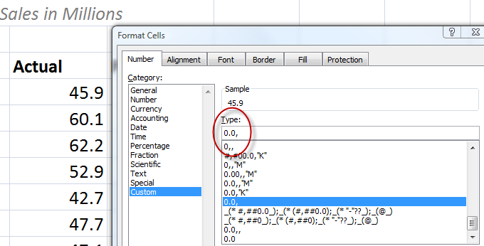
For example, instead of presenting this level of precision – 19, 699, 499, you can use this custom number format – 0.0,,”M”, to present this as 19.7M. From my perspective as both a presenter and an audience member, I prefer to see 19.7M. This makes it easier for me to process the information as an audience member. This makes it easier for me to present – saying 19,7 million is a lot easier than trying to say 19 million, 699 thousand, 4hundread and 99 dollars!

What is your preference?

Watch this short, focused Excel training video lesson to learn how to format and display large numbers in Excel so that you can make it easier for your audience to understand and act on the information that you are presenting.

Learn how to “Master Excel in Minutes – Not Months!”

Follow this link to watch this video lesson in High Definition, Full-screen mode on my YouTube Channel – DannyRocksExcels