How to Identify and Then Delete Duplicate Records in Excel

Identify & Delete Duplicates

Identify & Delete Duplicates

It is almost inevitable that, over time, your Excel data set will contain duplicate records. This can be costly – if the duplicate records are in your mailing list. And it can also result in errors when you count and calculate data.

Three Methods to Identify and Delete Duplicate Records

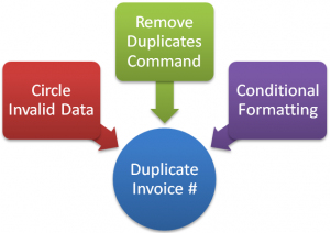
In this Excel Tutorial, I demonstrate three approaches to identify duplicate records in a data set:

  1. Circle Invalid Data – This tool works in coordination with Data Validation.
  2. Remove Duplicates – This powerful command was introduced in Excel 2007. It does not “preview” the records to be deleted, so my advice is to use this command with a copy of your data.
  3. Conditional Formatting – Greatly improved for Excel 2007 and Excel 2010. Now, you have a menu choice to apply conditional formatting to either Duplicate or Unique Records. If you are still using Excel 2003 or earlier, I show you how to write the formula needed to use Conditional Formatting to highlight duplicate records.

Watch The Tutorial in High Definition on YouTube

Follow this link to view this Excel Tutorial in High Definition on my YouTube Channel – DannyRocksExcels
How to Take Advantage of Excel 2007 – 2010 Tables and Excel 2003 Lists

Excel Table Styles

Excel Table Styles

In this video tutorial, I cover multiple versions of Excel. I demonstrate how to take advantage of the Table Tools that were introduced in Excel 2007 and I also show you how to create Excel 2003 Lists.

Topics Covered on Video Tutorial

  • Convert a range of data to an Excel 2007, Excel 2010 Table.
  • Convert a range of data to an Excel 2003 List.
  • View and change the Total Row in each version of Excel.
  • Append new records to Tables and Lists.
  • Add a new field to Tables and Lists.
  • Write a formula in one cell of an Excel Table and have it automatically copy down for each record.
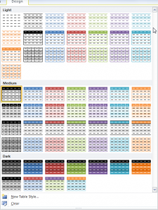
  • Change the Table Styles in Excel 2007 and 2010.
  • Use Conditional Formatting to add alternate row shading to an Excel 2003 List

Watch Video in High Definition on YouTube

Follow this link to watch this Excel Video Tutorial in High Definition on my YouTube Channel, DannyRocksExcels

Download This Excel Workbook

Click on this link to download the Excel Workbook that I used in this video tutorial.

Get my best-selling DVD-ROM, “The 50 Best Tips for Excel 2007” for only $39.95!

How to Apply Conditional Formatting to a Pivot Table in Excel

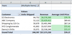
A Pivot Table is a great way for you to summarize and present the information contained in your data set. When you apply conditional formatting to your Pivot Table, you can “visually” spot important trends or anomolies in your data.

Improvements to Conditional Formatting

Conditional Formatting in Pivot Table

Condition Formatting for Above Average

Beginning with Excel 2007, Conditional Formatting has been dramatically improved. In addtion to pre-built formula rules, you can also apply Data Visualizations (Icon Sets, Data Bars and Color Scales).

Conditional Formatting for Above Average

In this lesson, I apply the pre-built “Above Average” rule. I want Excel to dynamically format the summary values that answer, “TRUE” to this question: “Is this value “Above the Average” in the range of cells selected?

This is the key to understanding how Conditional Formatting works. Special Formatting is applied only when the answer to your CONDITION (a rule or a formula) is TRUE.

Dynamically Filter Conditional Formatting

In this lesson, I use the Report Filter zone in my Pivot Table to see how conditions change when I change the time period in my report. Values that meet the Condition, “Above the Average,” receive the formatting that I established in my rule. Try this on your Pivot Table. It is a wonderful tool to use in an Excel Dashboard.

View This Video Tutorial in High Definition

Follow this link to watch this lesson in High Definition on my YouTube Channel, DannyRocksExcels.

My Extended Length Pivot Table Video Tutorials

I offer “free of charge,” a 24 minute in-depth video tutorial for creating your first Pivot Table in Excel. Follow this link to learn how to view it online or to download it to your computer.

Vist My New Online Shopping Site

My new, secure online shopping website – http://shop.thecompanyrocks.com/ – is now open. I invite you to visit and learn more about the new products that I have added.

How to Find and Change Numbers Stored as Text in Excel

Whenever a client or a colleague sends me an Excel workbook I like to inspect it, to be sure that the “numbers are really numbers.” I will not get accurate results when I SUM them if there are some cells that appear to contain numbers, but really display a “number stored as text.”

Prevent GIGO

Prevent GIGO

This is an example of GIGO – “Garbage in delivers Garbage Out!” I take steps to prevent an outbreak of GIGO in my Excel worksheets.

Looking for Numbers Stored as Text

As a best practice, I use both the COUNT() Function and the COUNTA() function to see if there is a difference between the number of cells with numbers (the COUNT Function) and the number of non-blank cells (the COUNTA Function). In this example, I was expecting to see 31 cells with numbers in the range of sales. There were on 27. So, I need to find those 4 cells that contain “numbers stored as text.” 

If you have a keen eye – and some time to spare – you can look for cells with a little Green triangle in the upper left corner. Click on the message next to these “marked” cells and read the error message. Excel will offer to correct the error – one cell at a time. That is not an efficient way to proceed!

Use the ISTEXT() or ISNUMBER() Functions

An alternative way to find the cells that contain text stored as numbers is to use one of the “logical functions” ISTEXT or ISNUMBER. Each returns either TRUE or FALSE when evaluating a cell. You can then sort the data to group the TRUE results together and then change them – again, one at a time. This is also not the best way to make the changes.

Use Conditional Formatting to Highlight Cells with Number Stored as Text

I like to use the ISTEXT() Function as a “Rule” to apply special formatting to the cells that evaluate as TRUE with Conditional Formatting. Be sure that you select the cells that you want to evaluate before applying the Conditional Formatting.

Use Paste Special – Add

The quickest way to change numbers stored as text into real numbers is to use Paste Special – Add. First, select and copy a blank cell. Next, select your data range – in this case the cells with “Sales.” Then, right click the selection and choose Paste Special. In the dialog box select “Add.” Now – instantly – all of the cells with numbers stored as text have been changed into real numbers. You have stamped out GIGO!

Learn how to “Master Excel in Minutes – Not Months!”

Follow this link to watch this video in High Definition, Full-screen mode on my YouTube Channel – DannyRocksExcels
How to Find and Delete Duplicate Records in Excel 2007

It is easy  – much too easy – to allow duplicate records to creep into an Excel database. Fortunately, starting in Excel 2007, it is really easy to first find and then delete duplicate records.

Remove DUplicate Records

Remove Duplicate Records

With the price of postage climbing, you cannot afford to send duplicate copies of a mailing piece. Not to mention that doing so reflects poorly on your company’s organizational skills. Likewise, having duplicate account entries makes for extra work and confusion.

Use Conditional Formatting to Highlight Duplicate Records

Starting in Excel 2007, Conditional Formatting got a lot easier to use. One of the menu selections is “Show Duplicate Records.” Now, with just a few mouse clicks, you can format the records that show duplicate values in your data set. I like to use this technique prior to acutally duplicating records so that I can get a sense of the number of possible duplicate records in my data set.

Selecting Duplicate Records to Delete

As a best practice, I always make a backup copy of my data set before I actually delete records. This way, I can quickly recover from any accidental deletions of non-duplicate records. When you choose the command to “Remove Duplicates,” a dialog box opens to reveal each field in your data set. Generally, you want to select all of the fields to narrow down the list of records to delete. Since I have already previewed the possible duplicate records by using Conditional Formatting, I have a pretty good idea of how many records will be deleted. You do not see a preview of the exact records that will be deleted, so make sure that you have a backup copy of your original list in order to restore any “accidental” deletions.

These new commands and menus introduced in Excel 2007 make deleting duplicate records a very quick process. Use them – wisely – to save yourself time, confusion and money!

Learn how to “Master Excel in Minutes – Not Months”

Watch this video lesson in High Definition, Full Screen mode. Follow this link to view this on my YouTube Channel – DannyRocksExcels

Secure Shopping Cart

Secure Shopping Cart

This is one of the tips that I offer on my DVD, “The 50 Best Tips for Excel 2007.” CLick here to open a secure shopping cart to purchase it.

How to Use Conditional Formatting to Compare Two Excel Lists

Clients and viewers frequently ask me to help them to compare two differeny lists in Excel. They want to find – or highlight – the values that are different in each list. For example, which customers appear in the 1st list but NOT in the 2nd list. So, I created this video lesson to demonstrate how to do this with Conditional Formatting.

In an earlier Excel Video Lesson, I demonstrated how to compare two Excel lists using either the MATCH() Function or the VLOOKUP() Function.

Conditional Formatting Rule

Conditional Formatting Rule

Use Conditional Formatting

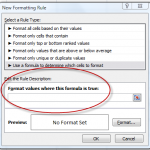
I demonstrate how to use Conditional Formatting to Highlight the Cell Values that are different when you compare two Excel Lists. I will use a “New Rule with a Formula” that must return the answer TRUE, to trigger the special formatting.

In Conditional Formatting, you first establish a “condition” that can be answered as either TRUE or FALSE. Then, for those cells where the answer to the condition is TRUE. the special “cell formatting” that you chose will apply.

In this lesson we will be using this Formula: =COUNTIF(List 2, 1st cell in List 1) = 0.

Steps to follow:

  1. Select the cells that you want the Conditional Formatting to apply to- in our example List 1.
  2. On the Home Tab of the Ribbon, click the Conditional Formatting arrow and select New Rule.
  3. Select New Rule – “Use a Formula to determine which cells to format.”
  4. Enter the formula – e.g. =COUNTIF(Range, Criteria) = 0 where the “Range” is the list of values in List 2 (Absolute Reference) and the “Criteria” is the 1st cell reference in List 1 (Relative Reference).
  5. Choose the Format for the cells when the condition is met – the result is TRUE. In this example, I choose to “FILL” the cells with a Blue background color.

Want to watch this video in High Definition, Full-Screen Mode? Click here to go to my YouTube Channel, DannyRocksExcels

Learn to “Master Excel in Minutes – Not Months!”

How to Add a Check Box Control to an Excel Form

Judging by the comments that I get from many clients, adding a “Check Box Control” to and Excel Form is not as easy as it appears at first glance.

And, I agree! I, too, struggled with adding Form Controls in Excel. Most of the explanations that I read seemed to add more confusion than clarification!

Spin Buttons in Excel

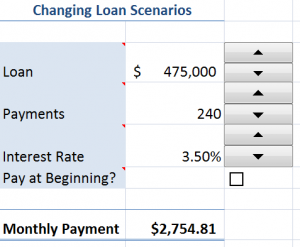
Spin Button Controls

That is why I created this Excel Training Video: to  lead you through the process; to save you some time and to ease your frustration.

Key Points to Remember:

  1. In Excel 2007, be sure to display the “Developer Tab” on the Ribbon in order to to Insert any Form Control.
  2. Choose the Controls in the “Forms Controls” and NOT in the Active X Controls.
  3. After you “draw” the Control Box on your Form, be sure to select a “Cell Link” to enable the Check Box Control.
  4. Remember that a Check Box Control can only be applied when the result of the Formula or Option is a Logical Value – either a result of  “True or False.”

Don’t be scared off! I find that this is an Excel concept that is better presented “visually.” I struggled for some time when I “read” how to add form controls.

So … I welcome your thoughts – “True or False.” Did I make this easy for you to understand?

Please feel free to add your comments below!

Watch My Video on YouTube

Follow this link to watch my tutorial on my YouTube Channel – DannyRocksExcels

Watch Video Now


Master Excel in Minutes Training Resources

I have created a series of extended length Excel Training Videos. I invite you to visit my secure online shopping site to:

Learn how to “Master Excel in Minutes – Not Months!”

Visualizing Your Data in Excel 2007

Excel 2007 makes it easy to “visualize” your data – directly in the cells of your worksheet! You do not need to take the time and effort to create a chart to visually represent your information.

You just take advantage of the tools in the newly-engineered Conditional Formatting command in Excel 2007. In this lesson I show you how to visualize your data as:

  • Data Bars – you get the equivalent of a Bar Chart drawn inside the data cells.
  • Icon Sets – pick from groups of 3, 4 or 5 Icon sets – for example, to show the data in the top third of your data range.
  • Color Scales – to add gradations of colors as numbers increase or decrease.

If you liked this tip and my style of Excel training, I invite you to visit my online store to purchase my DVD, “The 50 Best Tips for Excel 2007.”

You can view and download this Excel video lesson – for free – as a Podcast. Follow this link to visit my Podcast, Danny Rocks Tips and Timesavers” at the iTunes store.

You can also watch this Excel video lesson on YouTube.

Related Excel Videos:

3 reasons to apply conditional formatting to your Excel data

In my experience, Excel’s “conditional formatting” is an underutilized feature in spreadsheet analysis. And that is a shame. In this Excel training video, I will show you how, when and why to apply conditional formatting to dynamically point out important data in your spreadsheet.

Here are the steps to follow in this video lesson:

  1. Select the cells that you want to apply conditional formatting to. From the Format menus choose Conditional Formatting.
  2. In the dialog box choose “Cell Value is” and then choose an operator (Greater than, etc.) and then either type in a value or refer to a cell. This applies your Condition.
  3. Next, choose what Formatting to apply when cells meet your Condition(s). Click OK
  4. You may also choose, “Formula is” and then type in your formula to establish the Condition. Only use Formulas that can be answered as “TRUE” or “FALSE.” If the answer (implied or explicit) is “TRUE,” then the Conditional Formatting will apply.

Find the Excel Training Video that you want – Index to all Excel Topics

News! My DVD, “The 50 Best Tips for Excel 2007” is now availabe to purchase. I invite you to visit my online bookstore for more details.

Related Videos