I have published several video tutorials on the topic of Highlighting and Deleting Duplicate Records in Excel. However, a viewer recently asked me how to highlight cells that contain different values in the same Row. This is not as “crazy” as it first seems.
Scenario for this Tutorial
I am trying to determine accurate inventory counts for my product line. I have the count that the computer shows. I also have records from three different auditors who have performed manual counts. I need to easily highlight the cells where the inventory count “is off.” That is where there is a discrepancy between what the computer shows and what a manual count shows.
Go To Special Dialog Box
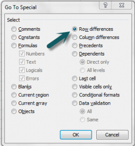
The commands in the Go To Special Dialog Box are some of my favorite tools. In my experience, I have found that most Excel users have never explored this dialog box. I think that will change after you watch this video tutorial. For the Row Differences tool, you first select the range of cells that contain your data – beginning with the left-most column. The Row Differences will use this left-most column as the “baseline” and highlight each cell in that row that contains a value that is different from this baseline.
Sorting & Filtering by Color
Beginning with Excel 2007, you can Sort by Color and you can also Filter by Color. After the cells were highlighted with the Row Differences command, I applied a background cell color to each highlighted cell.
Use one of my favorite Keyboard Shortcuts, Ctrl + Shift + L, when working with Filters in Excel 2007 or Excel 2010.
Watch this Excel Tutorial in High Definition
You can watch this tutorial in High Definition on my YouTube Channel – DannyRocksExcels. Click on this link to watch this video now.
Video Tutorials for Highlighting Duplicate Records
I mentioned that I have published many Excel Tutorials on the Topic of Highlighting & Removing Duplicate Records. Here are links to my tutorials:
- How to Find and Delete Duplicate Records in Excel 2007
- How to Identify and then Delete Duplicate Records in Excel
- How to Prevent Duplicate Entries in Excel with Data Validation
Shop for Excel Training Resources
I invite you to visit my secure online shopping website – http://shop.thecompanyrocks.com – to examine and purchase the many training resources that I offer.
Watch My Video Podcasts on iTunes
Click on this link to watch my “Danny Rocks Tips and Timesavers” video podcast on iTunes. – It is free of charge!
Note: The original Podcast Video did not have the correct video settings. This video has now been updated.
 How to Highlight Different Values in a Row in Excel [ 4:34 ] Play Now | Play in Popup | Download (2169)


