Tips for Working with Array Formulas and Functions in Excel

Using ARRAY Functions in Excel

ARRAY Formulas in Excel

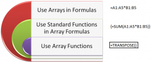
Array Formulas and Functions are very powerful tools to use in Excel. However, the concept of working with ARRAYs take a little bit of time and practice. In this video tutorial, I demonstrate how to:

  1. Create formulas that use ARRAYS as arguments
  2. Work with ARRAY FUNCTIONS – for example, the TRANSPOSE Function
  3. Key “Got’cha” steps to master – for example, selecting all cells to receive formula results before creating the ARRAY Formula.
  4. The importance of using Ctrl+Shift+Enter to complete the Array formula.

What is an ARRAY?

“An Array is a collection of Cells or Values that Excel treats as a single unit.”

Why Use an ARRAY Formula?

  1. Automatic Level of Protection for Formula Cells – You cannot delete nor edit a single cell in an Array Formula
  2. Eliminate Intermediary Calculations – For example, you can find the Grand Total without having to create a field to calculate “Extended Price.”
  3. Worksheet, usually, calculates faster because you are using fewer formulas.

Visit My NEW Online Shopping Website

http://shop.thecompanyrocks.com is my new, secure online shopping website. I invite you to visit and preview my new products.

Watch Tutorial in High Definition

Follow this link to view this tutorial in High Definition on my YouTube Channel – DannyRocksExcels

How to Use an Excel Data Table for “What-if” Analysis

Excel has many tools that give you answers to “What-if” questions. An Excel Data Table allows you to feed a series of “substitute values” into two arguments in a formula. For example, with a Data Table you can:

  • See a table of monthly payments on a loan by substituting both the “Interest Rate” and the “Amount Borrowed” simultaneously.
  • See a table of “Net Payments” by changing both the “Sales Price” and the “Quantity” simultaneously.
  • See the amount that you “tip” a service professional by changing both the “Tip Percentage” and the “Food Total” simultaneously.

As you will see in this Excel Video Lesson, the trick is to understand which series of values are the “Row Inputs” and which series of substitute values are the “Column Inputs.”

Trust me on this: It is easier to “see” how to set up a Data Table than it is to “write a description” of a Data Table. So, I invite you to “see for yourself” how easy it is to set up an Excel Data Table and get answers to two simultaneous “What-if” questions!

Click here to see a Listing of “The 50 Best Tips for Excel 2007.”

Learn how to “Master Excel in Minutes – Not Months!”

Perform "What-if" analysis with a 2 input Data Table

Here are the steps to follow in this video lesson:

  1. Create a formula that references cells – e.g. =PMT(B4/12,B5,B3)
  2. To the right of this formula cell, enter a series of “substitute” values – e.g. 36, 48, 72 months.
  3. Directly below the formula cell, enter another series of “substitute” values – 4%, 4.5%, 5%, etc.
  4. Select the range of cells for the Data Table – starting with the formula cell.
  5. From the Excel Menu, choose Data, Table.
  6. For the “Row Input Cell,” click the cell in the original formula for which you want to “substitute” the row values in your Data Table.
  7. For the “Column Input Cell,” click the cell in the original formula for which you want to “substitute” the column values in your Data Table. Then click OK.

NEW! Download the Excel Workbook that I Use in this Video:

Find the video lesson that you want – Index to all Excel Topics

News! My DVD, “The 50 Best Tips for Excel 2007” is now available to purchase. I invite you to visit my online bookstore for more details.