How to Use Text Functions in Excel

Text Functions in Excel

Text Functions

In my experience, I find that many of my clients do not realize that Excel has many powerful – and easy to use – Text Functions.

Even more amazing, I observe clients spending hundreds of hours and thousands of dollars “re-keying” or “manually editing” text entries that have been downloaded from a Main Frame Computer. If you – or your colleagues – have been doing this, you will want to watch this Excel Video Tutorial.

Categories of Text Functions in Excel

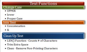
In this Excel video lesson, I demonstrate how to use three categories of Text Functions:

  1. Transform Text – Use the UPPER, lower and Proper functions to change the “Case” of a text string.
  2. Join Text – Use either the CONCATENATE() Function or the & (Ampersand) Operator to join two or more text strings into a single text string.
  3. Clean-up Text – Use the LEN(), TRIM() and CLEAN() Text Functions to “trim the fat” from text strings – especially those that you download from a Main Frame Computer.

Once again, in my experience, I have too many clients contacting me in a panic because they get a REF# error when using Text Functions. I demonstrate how to recover from a “seeming disaster” and also how to use COPY – PASTE SPECIAL – VALUES to transform Formulas into Constant Values.

I welcome your feedback. Please send me an email: danny@thecompanyrocks.com – to let me know if this tip helped you to save time and money. I also welcome your suggestions for future Excel Video Lessons to create and post here, on my website.

Watch This Excel Video Tutorial in High Definition Mode

Follow this link to view this Excel Video Lesson in High Defintion Mode on my YouTube Channel – DannyRocksExcels

Download the Excel Workbook

Follow this link to download the Excel Workbook I use in this lesson.

Learn How to Master Excel in Minutes – Not Months!

If you like this Excel Video Tutorial, I invite you to learn more about the resources that I offer to help you to improve your Excel skill set.
How to Lookup a Value Using Multiple Columns in Excel

There are times when the VLOOKUP Function will not return the value that you want to lookup. Suppose, for example, that you need to lookup the “Title” for an employee where the First Name and Last Name are in separate columns. A VLOOKUP() will not help you in this example. Let me show you how to accomplish this.

Key Concepts Covered

  • Use the “&” (Ampersand) to Join two cells that contain Text Values
  • Use the Index() and Match() Functions for the Lookup
  • Create an Array Formula to perform the Lookup – Use “Ctrl+Shift+Enter” with Array Formulas
  • Create and use “Named Cell Ranges” in your formulas to make it easier to enter and understand the formula

Be sure to check out all of the other Excel Video Lessons on Lookups. Click here to go to the Archive of Lookup Function Videos.

I invite you to subscribe to my “Danny Rocks Tips and Timesavers”Video Podcast on iTunes – it is free!

You can learn how to “Master Excel in Minutes!”

How to Prepare Your Zip Codes for Mailing Labels

Clients call me up in a panic. “Danny, we are sending out a direct mail piece and Excel has screwed up our Zip Codes – they only contain 4 numbers! The Post Office can’t deliver the mailing piece this way. Can you help us?”

Yes I can!

The problem is not with Excel. The problem is not choosing the correct formatting for the Columns / Fields that contain Zip Codes or Postal Codes.

At the risk of jeopardizing some lucrative consulting fees, I will demonstrate how to solve this problem in this short Excel Video Tutorial.

Here are the steps to follow in this Excel Video Lesson:

  1. When you have control over your data, pre-format your Zip Codes column using the “Formant Cells, Number, Special, Zip Code” format.
  2. If your data contains cells with both 4 and 5 digit Zip Codes, use this formula:
  3. =IF(A2<=9999, 0&A2, A2)
  4. Now, you will see some cells formatted as “Text” – aligned to the Left side of the cell and other cells formatted as “Numbers” – aligned to the Right side. Take the next step:
  5. First, Copy the data (the cells w/ the =IF() Function) and choose Paste Special, Values to return the results of the formulas.
  6. With the cells still selected choose, Data, Text-to-Columns and choose “Fixed Length.” After previewing your data, choose the “Format as Text”  button and Finish the Wizard.

Find the Excel Training Video that you want – Index to all Excel Topics

News! My DVD, “The 50 Best Tips for Excel 2007” is now availabe to purchase. I invite you to visit my online bookstore for more details.

Learn 2 ways to combine text from multiple cells into 1 cell

Here are the steps to follow in this lesson:

  1. Method #1 – Use the =CONCATENATE() Function Wizard.
  2. Text1 will be the cell reference for “First Name.”
  3. Text2 will indicate a SPACE between the 2 names. Type ” ” into the text2 indicator.
  4. Text3 will be the cell reference for “Last Name.”
  5. Method # 2 – Use the Ampersand (&) symbol in your formula e.g. =B4&” “&C4.

Find the video lesson that you want – Index to all Excel Topics

News! My DVD, “The 50 Best Tips for Excel 2007” is now available to purchase. I invite you to visit my online bookstore for more details.

Related Video Lessons