Clients and viewers frequently ask me to help them to compare two differeny lists in Excel. They want to find – or highlight – the values that are different in each list. For example, which customers appear in the 1st list but NOT in the 2nd list. So, I created this video lesson to demonstrate how to do this with Conditional Formatting.
In an earlier Excel Video Lesson, I demonstrated how to compare two Excel lists using either the MATCH() Function or the VLOOKUP() Function.
Use Conditional Formatting
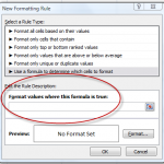
I demonstrate how to use Conditional Formatting to Highlight the Cell Values that are different when you compare two Excel Lists. I will use a “New Rule with a Formula” that must return the answer TRUE, to trigger the special formatting.
In Conditional Formatting, you first establish a “condition” that can be answered as either TRUE or FALSE. Then, for those cells where the answer to the condition is TRUE. the special “cell formatting” that you chose will apply.
In this lesson we will be using this Formula: =COUNTIF(List 2, 1st cell in List 1) = 0.
Steps to follow:
- Select the cells that you want the Conditional Formatting to apply to- in our example List 1.
- On the Home Tab of the Ribbon, click the Conditional Formatting arrow and select New Rule.
- Select New Rule – “Use a Formula to determine which cells to format.”
- Enter the formula – e.g. =COUNTIF(Range, Criteria) = 0 where the “Range” is the list of values in List 2 (Absolute Reference) and the “Criteria” is the 1st cell reference in List 1 (Relative Reference).
- Choose the Format for the cells when the condition is met – the result is TRUE. In this example, I choose to “FILL” the cells with a Blue background color.
Want to watch this video in High Definition, Full-Screen Mode? Click here to go to my YouTube Channel, DannyRocksExcels
Learn to “Master Excel in Minutes – Not Months!”
 How to Use Conditional Formatting to Compare Two Excel Lists [ 8:33 ] Play Now | Play in Popup | Download (1495)


Hi! interesting, you can go here to know how to make conditional lists:
http://runakay.blogspot.com/2011/03/conditional-lists-on-excel.html
To compare two sorted lists (each of one column), the following works.
Create column ranges range1 and range2 in the worksheet(s).
Sort both range1 and range2 (along with other relevant columns).
Use the following as conditional formatting formulas:
=IFERROR(INDEX(range1,MATCH(RC1,range1,TRUE)),0)RC1
=IFERROR(INDEX(range2,MATCH(RC1,range2,TRUE)),0)RC1
RC1 means that you are formatting the 1st column.
You CANNOT just use RC here, but must specify the column.
This magic formula works beautifully. Each range will highlight all values NOT FOUND in the other. If you want to reverse this so as to highlight values that ARE FOUND, just change “” above to “=”