How to Perform Time Period Calculations in Excel

Time Calculations in Excel

Time Calculations in Excel

Judging by the number of calls that I get from my viewers, working with Time Period Calculations is one of the most problematic challenges in Excel. My goal for this tutorial is to demonstrate how you can easily avoid the frustrations when you calculate elapsed time and total a series of time – e.g. hours worked during the week.

Apply a Custom Format to Formula Cells

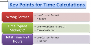
When you create an Excel Formula that subtracts a Start Time from an End Time, you are likely to get a result that looks like 2:30 AM. This is not what you want to see! The solution is to apply a Custom Time Format – e.g. h:mm – to the formula cell(s).

Time that “Spans Midnight”

Many people work the “Graveyard Shift.” The start work late in the evening and they end work early the next morning. The problem that occurs when you want to calculate the number of hours worked is that Excel believes that you are performing a “negative time” operation and the result is a cell filled with ######## (Hash Marks). This happens because Excel thinks that both the Start Time and the End Time belong in the same day. To solve this, you could use an IF() Function formula. However, there is a much easier formula to use as I demonstrate in this video. It uses the MOD() Function.

Total Hours Worked

Use the SUM() function to total 8:00 hours worked each weekday. You are expecting to see 40:00 hours worked. So why does Excel return 16:00 hours instead? By default, Excel interprets 24:00 hours as a single day. So it subtracts 24:00 from the 40:00 hours worked to return 16:00 hours. Unless you make a formatting change to the formula cell you are going to have many unhappy and under paid employees.

The solution? Apply the [h]:mm Custom Formatting to the Formula Cells. Amazingly enough, Excel does not include [h]:mm as one of the Custom Formats in the list. So, simply edit one of the other formats and you will now have the correct answer displayed for your formula!

Learn More Tips for Excel

I invite you to visit my secure online shopping website – http:shop.thecompanyrocks.com – to preview all of the resources that I offer including “The 50 Best Tips for Excel 2007” DVD-ROM.

Subscribe to the “Danny Rocks Tips and Timesavers” Video Podcast on iTunes

I offer a free video podcast for many of my video tutorials at the iTunes Store. Follow this link to see all of the Podcasts that I have posted. If you like what you see, I invite you to subscribe to this free service.

Watch Tutorial in High Definition

You can view this tutorial in High Definition on my YouTube Channel – DannyRocksExcels.


Share and Enjoy:
  • Add to favorites
  • Facebook
  • Twitter
  • Technorati
  • Print
  • email
  • Digg
  • StumbleUpon
  • del.icio.us
  • Yahoo! Buzz
  • Google Bookmarks
  • Orkut
  • SphereIt
  • Sphinn

How to Protect Cells that Hold Formulas in Excel

Protect Cells w Formulas

Protect Excel Formula Cells

Learning how to Protect the Excel Worksheet Cells that contain Formulas is a three-step process. This process tends to confuse and frustrate many Excel users. Some of the steps seem counter-intuitive when you first begin the process. That is why I created this video tutorial – To demonstrate each of the steps; to remove the confusion.

First, I show you how this is done in Excel 2010 / Excel 2007. Next, I show you how to protect the Formula Cells in Excel 2003.

Key Concept for Protecting Formula Cells

By default, all cells in an Excel Workbook are “Locked!”

So, if you are going to allow a user to input current values in the worksheet, you must first “select” the input cells and then, “Unlock” them.

Protecting Excel Worksheet

The final step in the process is to Protect the Worksheet. I rarely use a password for the worksheet because I tend to forget it and then I cannot even access the protected worksheet!

Take care in the Protect Sheet Dialog Box to select only the options that best suit your purpose. For example, in this video tutorial, I choose to limit users to select only the cells that I unlocked in steps 1 and 2.

Go To Special Dialog Box

The quickest way to select the cells that you wish to “unlock” is to open the Go To Special Dialog Box. There, choose “Constants.” You can limit the constants to “Numbers” as I do in this tutorial.

Danny Rocks Tips and Timesavers Podcast on iTunes

I invite you to subscribe to my “free” video podcast on iTunes. Click on this link to access all of my Podcast Videos.

Watch Tutorial in High Definition

Follow this link to view this Excel Tutorial in High Definition on my YouTube Channel – DannyRocksExcels


Share and Enjoy:
  • Add to favorites
  • Facebook
  • Twitter
  • Technorati
  • Print
  • email
  • Digg
  • StumbleUpon
  • del.icio.us
  • Yahoo! Buzz
  • Google Bookmarks
  • Orkut
  • SphereIt
  • Sphinn

Summarizing Employee Hours Worked and Vacation Time over 52 Weeks in Excel

Sum Across Worksheets

Sum Across Worksheets

This is the third episode in my series of Excel Tutorials where I share my best practices for creating an Excel Workbook that contains 52 weeks of Employee Time Cards. In this lesson, I focus on techniques to Summarize – or Consolidate – the hours worked or taken as vacation, by each employee, over a period of several weeks.

Sum Across Worksheets

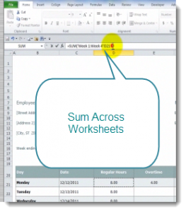
This is a great tip to learn! In my experience, I find that very few experienced users of Excel know that you can do this! This will eliminate the hassle of linking to a cell in individual worksheets to create your formula. There is, after all, a limit to the number of characters that you are allowed in a formula!

Consolidate Data By Position

Since each worksheet in this workbook is identical in structure, Data Consolidation is simple. Provided, that is, that you remember to “Add” each worksheet range reference in the Dialog Box. In this example, I have “created a link” to each worksheet so that the data can be easily updated.

Links to Other Tutorials in this Series

Shop for Additional Resources

I invite you to visit my new, secure online shopping website – http://shop.thecompanyrocks.com – where you can preview all of the resources that I offer you.

Watch Tutorial in High Definition

Follow this link to view this Excel Tutorial in High Definition on my YouTube Channel – DannyRocksExcels

Share and Enjoy:
  • Add to favorites
  • Facebook
  • Twitter
  • Technorati
  • Print
  • email
  • Digg
  • StumbleUpon
  • del.icio.us
  • Yahoo! Buzz
  • Google Bookmarks
  • Orkut
  • SphereIt
  • Sphinn

How to Use the New Natural Language Date Filters in Excel

Natural Language Date Filters

Natural Language Date Filters

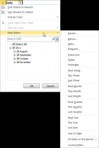
Recently, one of my viewers asked me to go into greater detail in demonstrating how the new Natural Language Date Filters work in Excel. Natural Language Filters were introduced in Excel 2007 and they are a great tool to use! Now, instead of writing complex formulas as criteria in Advanced Filters, you can simply click, “Yesterday” to see all of the records from the previous day!

Of course, you must actually have records in your data set for that date!

The Natural Language Date Filters are related, by position, to TODAY(). The TODAY() Function is a “Volatile Function” that returns the value for the current date as found in your computer systems internal clock. The result of the TODAY() Function will change each day. And so, by definition, will the result for a “Yesterday” filter!

Filter for Specific Date

There are several methods that you can use to filter for a specific date or range of dates. One method that I demonstrate in this tutorial is the “Custom Date” dialog box.

Watch Tutorial in High Definition

Follow this link to watch this Excel Tutorial in High Definition on my YouTube Channel – DannyRocksExcels

Learn About My New Extended Length Video Tutorials

I have recently released a series of extended length (90 minutes) video tutorials. They are part of my “Master Excel in Minutes” Series. Each video focuses on one topic. My first video is focused on Excel Pivot Tables. I have created Videos for Excel 2010, Excel 2007 and for Excel 2003. You also have the choice of purchasing the video for immediate downloading or shipped to you on a DVD-ROM.

Follow this link to go to the information page for my “Master Excel in Minutes” video tutorial series.

Share and Enjoy:
  • Add to favorites
  • Facebook
  • Twitter
  • Technorati
  • Print
  • email
  • Digg
  • StumbleUpon
  • del.icio.us
  • Yahoo! Buzz
  • Google Bookmarks
  • Orkut
  • SphereIt
  • Sphinn

How to Automatically Add a Time / Date Stamp Whenever You Add or Edit a Record in Excel

VBA Code to add Time Stamp

VBA Code to add Time Stamp

In this video tutorial, I respond to one of the most frequent requests that I get from my viewers – “How do I automatically add a ‘Time / Date Stamp’ whenever I add or edit a record in my Excel Worksheet?”

On the surface, this might appear to be a “simple” question to answer. However, I promise that you will be frustrated if you try to solve this problem by using the =NOW() Function or one or both of these Keyboard Shortcuts:

  • Ctrl + ; (Semi-colon) to add a Date Stamp
  • Ctrl + Shift + : (Colon) to add a Time Stamp

Because … NOW() is a “Volatile Function” that automatically updates to display – in all records that refer to NOW() – the current date and time. And … because, it is difficuly to automate the combination of Keyboard Shortcuts to apply a Date / Time Stamp.

So … what is the solution?

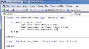
Use VBA to Create a Simple “Event Handler” Macro

Don’t get scared off! Don’t say, “I can’t write a VBA Macro!”

I PROMISE you – an Intermediate Level User of Excel – that by investing 10 minutes to watch this tutorial – that you WILL be able to automate this process to add a Time / Date Stamp whenever you add or edit a record in Excel.

I had you – the Intermediate / Early Advanced Level Excel user in mind when I created this video tutorial. I take you step-by-step through the process. I point out the potential “got’cha” steps. I am confident that I can help you to advance your skill set in Excel with this video tutorial!

Watch Tutorial in High Definition

I invite you to watch this Excel Tutorial in High Definition on my YouTube Channel – DannyRocksExcels

Visit My Online Shopping Site

I invite you to visit my new, secure online shopping site – http://shop.thecompanyrocks.com – to see all of the new products that I have created and offer for sale!

Share and Enjoy:
  • Add to favorites
  • Facebook
  • Twitter
  • Technorati
  • Print
  • email
  • Digg
  • StumbleUpon
  • del.icio.us
  • Yahoo! Buzz
  • Google Bookmarks
  • Orkut
  • SphereIt
  • Sphinn

Tips for Working with Array Formulas and Functions in Excel

Using ARRAY Functions in Excel

ARRAY Formulas in Excel

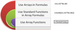
Array Formulas and Functions are very powerful tools to use in Excel. However, the concept of working with ARRAYs take a little bit of time and practice. In this video tutorial, I demonstrate how to:

  1. Create formulas that use ARRAYS as arguments
  2. Work with ARRAY FUNCTIONS – for example, the TRANSPOSE Function
  3. Key “Got’cha” steps to master – for example, selecting all cells to receive formula results before creating the ARRAY Formula.
  4. The importance of using Ctrl+Shift+Enter to complete the Array formula.

What is an ARRAY?

“An Array is a collection of Cells or Values that Excel treats as a single unit.”

Why Use an ARRAY Formula?

  1. Automatic Level of Protection for Formula Cells – You cannot delete nor edit a single cell in an Array Formula
  2. Eliminate Intermediary Calculations – For example, you can find the Grand Total without having to create a field to calculate “Extended Price.”
  3. Worksheet, usually, calculates faster because you are using fewer formulas.

Visit My NEW Online Shopping Website

http://shop.thecompanyrocks.com is my new, secure online shopping website. I invite you to visit and preview my new products.

Watch Tutorial in High Definition

Follow this link to view this tutorial in High Definition on my YouTube Channel – DannyRocksExcels

Share and Enjoy:
  • Add to favorites
  • Facebook
  • Twitter
  • Technorati
  • Print
  • email
  • Digg
  • StumbleUpon
  • del.icio.us
  • Yahoo! Buzz
  • Google Bookmarks
  • Orkut
  • SphereIt
  • Sphinn

Master Excel Pivot Tables in 90 Minutes: Announcing My New Extended Length Video Tutorials!

Master Pivot Tables in Minutes

Master Pivot Tables in Minutes

I am proud to announce the publication of my new series of “Extended Length” video tutorials: “Master Excel Pivot Tables in 90 Minutes!”

Now, you can can get an in-depth video tutorial, so that you can Master Excel Pivot Tables with 90 minutes of video instruction. You also receive the actual Excel Workbook file that I used while filming the video lessons as well as a printed step-by-step instructional manual.

What Makes this Product Unique?

  •  Excel Versions for the Video Tutorials

  • Available for Excel 2010, Excel 2007 or Excel 2003

Multiple Options for Delivery

Resources to Assist Your Learning

  • The Excel Workbook file that I used while filming each video lesson – Included with purchase!
  • PDF Manual of Step-by-Step Instructions – That you can print out – Included with purchase!

Take a Short Video Tour

Follow this link to watch a short – 5 minutes – video tour of my new products on my YouTube Channel – DannyRocksExcels

Visit My New Secure Online Shopping Website

I invite you to visit http://shop.thecompanyrocks.com This is my new online shopping website. I have created secure shopping carts to ensure that your privacy is protected. I also offer a 100% Customer Satisfaction Policy. If, for any reason, you are not 100% satisfied with any of my products, I will refund your purchase with no questions asked!

Danny Rocks

The Company Rocks

Share and Enjoy:
  • Add to favorites
  • Facebook
  • Twitter
  • Technorati
  • Print
  • email
  • Digg
  • StumbleUpon
  • del.icio.us
  • Yahoo! Buzz
  • Google Bookmarks
  • Orkut
  • SphereIt
  • Sphinn

How to Use the SOLVER Tool in Excel to Produce the Optimal Result for a Formula

Key Points for SOLVER

SOLVER in Excel – Key Points

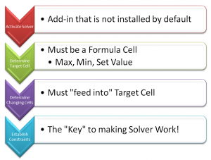
I am responding to a “flurry” of requests to produce an Excel Video Tutorial that demonstrates how to use the SOLVER TOOL in Excel. Here are the key points to remember when you want to use the SOLVER Tool:

Activate the SOLVER Tool

SOLVER is an “Add-in” tool that needs to be “activated” before you can use it. In Excel 2007 / 2010, you do this via Excel Options – Addi-Ins – Excel Options. In Excel 2003, you do this via the Tools Menu – Add-ins – Solver.

Prepare Data for Solver

In order to use the SOLVER Tool, you must:

  • Establish the “Target Cell.” This cell must contain a formula. This is the cell that you want to “optimize” by using SOLVER.
  • Determine the “By Changing” Cells. These are the cells that SOLVER will change in order to deliver the optimized result in the Target Cell. The “By Changing” cells MUST “Feed Into” the Target Cell.
  • Establish the CONSTRAINTS for SOLVER. This is the “key’ element that gives SOLVER its power. You can add as many constraints as needed. My recommendation is that you “write them out” before you start  to use the SOLVER Tool.

SOLVER is very powerful. However, you MUST “think it through” before you apply it. It will take lots of practice for you to understand how to properly set up your data to produce appropriate SOLVER results.

Part 2 in this Series of Tutorials for Solver in Excel

Here is the link to watch Part 2 in this Series of Tutorials about the SOLVER Add-in Tool in Excel

Download Excel Workbook for this Lesson

Follow this link to download the Excel Workbook that I used for this lesson. I store my uploaded Excel workbooks on my SkyDrive at www.office.live.com

View this Tutorial in High Definition

Click on this link to watch this Excel Tutorial in High definition / Full Screen Mode – on my YouTube Channel, DannyRocksExcels

Share and Enjoy:
  • Add to favorites
  • Facebook
  • Twitter
  • Technorati
  • Print
  • email
  • Digg
  • StumbleUpon
  • del.icio.us
  • Yahoo! Buzz
  • Google Bookmarks
  • Orkut
  • SphereIt
  • Sphinn

How to Prevent Duplicate Entries in Excel with Data Validation

Formula for Data Validation

Formula for Data Validation

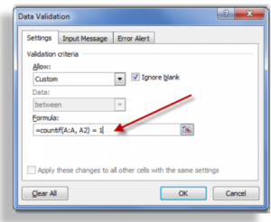
Over time, it is easy for duplicate entries to creep into an Excel Data Set. In this video tutorial, I show you, step-by-step, how to apply Data Validation to a range of cells so that anyone who attempts to enter a duplicate value will be prevented from doing so.

Use a “Logical Formula” for Data Validation

In this lesson, I show you how to “customize” the COUNTIF Function in the Data Validation Dialog Box so that it returns the value of TRUE. Logical formulas return either TRUE or FALSE. You MUST use a Logical Formula in Data Validation.

What Else is Covered in this Tutorial?

  • Use Paste Special – Validation to extend Data Validation to a wider range of cells
  • Use Find – Go to Special – Validation to highlight all cells on worksheet that contain Data Validation
  • Use Circle Invalid Entries from the Data Validation menu to automatically “draw a red circle” around existing cells that contain duplicate values
  • How to quickly remove Data Validation from a Range of Cells

Related Topic – Conditional Formatting in Excel

Another way to highlight existing cells that contain duplicate values is to use Conditional Formatting. The improvements in Excel 2007 and Excel 2010 make this “a snap” because this is now a Menu Selection! In my next tutorial, I will show you how this is done in both Excel 2003 – with the COUNTIF Function – and from the new Menu Selections introduced in Excel 2007.

Watch Tutorial in High Definition

Follow this link to my YouTube channel – DannyRocksExcels – where you can watch this tutorial in High Definition mode.

Share and Enjoy:
  • Add to favorites
  • Facebook
  • Twitter
  • Technorati
  • Print
  • email
  • Digg
  • StumbleUpon
  • del.icio.us
  • Yahoo! Buzz
  • Google Bookmarks
  • Orkut
  • SphereIt
  • Sphinn

Keyboard Shortcuts to Enter and Edit Data Efficiently in Excel


Keyboard Shortcuts to Enter Data

Keyboard Shortcuts to Enter Data

This is the latest installment in my series of video tutorials where I demonstrate how to use Keyboard Shortcuts in Excel. In this tutorial, I demonstrate how to Enter and Edit Data Efficiently in Excel using Keyboard Shortcuts.

Tips Covered on Video Tutorial

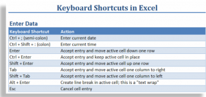
Here are the main Keyboard Shortcuts that I show you how to use on this video:

  • Enter Current Date in a cell.
  • Enter Current Time in a cell.
  • Use Ctrl + Enter to accept data entry and keep the focus on the current cell.
  • Use Ctrl + Enter to populate a range of selected cells.
  • Use Alt + Enter to “Wrap the Text” in a cell.
  • Use F2 to edit data inside a cell.
  • Use Ctrl + left & right directional arrows to move to the beginning of the next / previous word while editing in the cell.
  • Use ‘ (apostrophe) as the first character in a cell to make this a “text” entry.

Download my complete Chart of Popular Keyboard Shortcuts as a PDF 

 Follow this link to download – for free – my 5 Page Chart of Popular Excel Keyboard Shortcuts as a PDF.

Subscribe to my Video Podcast on iTunes

Here is the link to subscribe to my video podcast, “Danny Rocks Tips and Timesavers” on iTunes. It is offered for free!

Watch Tutorial in High Definition on YouTube

Follow this link to view this Excel Tutorial in High Definition mode on my YouTube Channel – DannyRocksExcels

Share and Enjoy:
  • Add to favorites
  • Facebook
  • Twitter
  • Technorati
  • Print
  • email
  • Digg
  • StumbleUpon
  • del.icio.us
  • Yahoo! Buzz
  • Google Bookmarks
  • Orkut
  • SphereIt
  • Sphinn