Date Functions And Formats In Excel

Danny September 11, 2012 1 Comment

How to Dynamically Color-Code Dates with Conditional Formatting in Excel

Conditional Formatting for Dates

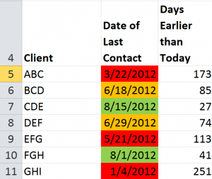
One of my viewers wants to learn how to “dynamically” color-code cells that contain dates. She is monitoring the frequency of contact with her clients and she wants Excel to automatically apply:

One background color to cells where it has been less than 60 days since last contact
A different color when the time frame is between 60 and 90 days
A third color when it has been over 90 days since the last contact with a client

Here, I demonstrate how she can do this using Conditional Formatting Rules. However, this will only work if you are using Excel 2007 or Excel 2010.

Understanding Dynamic Date Functions

In order to make this visualization “dynamic,” I make references to cells that contain the =TODAY() Function. This is a “volatile” function that updates automatically based upon the date in your computer system’s clock. I use this to classify the last date of contact with her clients.

Improvements in Conditional Formatting

Beginning with Excel 2007, you can now apply multiple rules that use formulas. Remember that when you use a formula, it must evaluate as “TRUE” in order to apply the formatting that you specify.

Formulas Used to Apply Conditional Formatting

Rules for Conditional Formatting

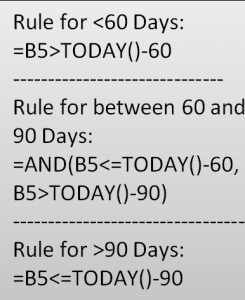
To make it easier for you to practice this skill, I have posted this table that details the formulas that I used for each of the three rules in my video tutorial.Note that with the middle condition, I use the =AND() Function. All logical tests must answer TRUE for the AND() Function to return TRUE.

It will take a little bit of practice for you to become comfortable with these formulas. As a Best Practice, I recommend that you create a table of formulas so that you can see how a “tweak” in your formula can turn a FALSE answer into a TRUE answer.

Watch this Video in High Definition

Follow this link to watch my Excel Tutorial in High Definition on my YouTube Channel – DannyRocksExcels

Get the Best Tips and Training for Excel

Click on this link to learn more about my best-selling DVD-ROM, “The 50 Best Tips for Excel 2007.” This link will take you to my secure online shopping website – http://shop.thecompanyrocks.com

Subscribe to my Video Podcast on iTunes

Here is the link to go to my free Video Podcast, “Danny Rocks Tips and Timesavers” on iTunes.

Share and Enjoy:

How to use Conditional Formatting to Color-Code Dates in Excel [ 8:49 ] Play Now | Play in Popup | Download (3143)

Danny July 8, 2012 1 Comment

How to Calculate the Calendar Year Quarter for a Date in Excel

Formulas to Calculate a Calendar Year Quarter

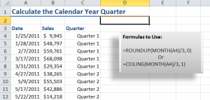
After watching my previous video tutorial, “How to Place Dates in a Fiscal Year Quarter,” several viewers requested that I demonstrate how to calculate the calendar year quarter for a date.

This requires “nesting” the MONTH() /3 Function inside either the ROUNDUP() or the CEILING() Function. I break these formulas down step-by-step in this video so that you can see how they work.

Formatting Numbers to Include Text

As a bonus, I demonstrate how to format the formula result cells to include the text “Quarter.” This is really simple to create as a custom format.

Download this Video Podcast from iTunes

You can watch and download this – and many of my – video tutorials for free at iTunes. Here is the link to my iTunes video podcast, “Danny Rocks Tips and Timesavers.”

Watch Video in High Definition

Follow this link to watch this Excel Tutorial in High Definition on my YouTube Channel – DannyRocksExcels

Visit my Secure Online Shopping Website

I invite you to visit my online shopping site – http://shop.thecompanyrocks.com – to preview and purchase my training resources. I guarantee your satisfaction 100%. I will refund your purchase if, for any reason, you are not satisfied with my products!

Share and Enjoy:

How to Calculate the Calendar Year Quarter for a Date [ 5:19 ] Play Now | Play in Popup | Download (1131)

Filed Under: Date Functions and Formats in Excel, Excel Date and Time Functions, Excel Functions, Excel Training, Format Cells in Excel, Podcast Tips & Timesavers Tagged: CEILING Function in Excel, Custom Formats for Numbers in Excel, Excel Video Training, MONTH Function, Nested Functions, Nesting Formulas and Functions, ROUNDUP Function, Video lessons for Excel

Danny July 1, 2012 1 Comment

How to Place Dates in a Fiscal Year Quarter

Many organizations operate in a Fiscal Year – for example, April 1 through March 31 of the next calendar year. I get many requests from viewers for help with placing calendar dates into the proper Quarter for their Fiscal Year.

While researching a question from one viewer, I cam across a very interesting formula that nests the “undocumented” DATEDIF() Function inside the CEILING() Function. I found this formula in the book, “Formulas and Functions with MS Excel 2003,” written by Paul McFedries. It is a very efficient formula.

What is Covered on the Video

Watch this video tutorial as I break down each step. As a Best Practice, I recommend that you break down a complex formula by working from the “inside out.” I start with the “nested” DATEDIF() function and then demonstrate the results of each formula detail.

Learn More About the “Undocumented” DATEDIF() Function

For various reasons, Microsoft does not offer any help or documentation for the very useful DATEDIF() Function. In fact, it is not even listed as a Function! However, it is very useful and often found in VBA (Visual Basic for Applications) coding. Here, are links to two videos that I created to help you understand how to use DATEDIF():

Learn How to Calculate a Calendar Year Quarter

In response to viewer requests, I created a companion video tutorial -” How to Calculate a Calendar Year Quarter in Excel.”

Resources Available at The Company Rocks

I invite you to visit my secure online shopping website – http://shop.thecompanyrocks.com – to preview the many resources that I offer for helping you to improve your software skills.

Watch Video Tutorial in High Definition

If you would like to watch my video tutorial for “Finding the Fiscal Year Quarter for any Date,” click on this link. I have posted it on my YouTube Channel – DannyRocksExcels

Watch this Video Now

Share and Enjoy:

Filed Under: Date Functions and Formats in Excel, Excel Date and Time Functions, Excel Formulas, Excel Functions, Excel Training Tagged: CEILING Function in Excel, DATEDIF Function in Excel, Excel Video Training, Fiscal Year Quarter, Nested Functions, Nesting Formulas and Formulas, Place Dates in Fiscal Year Quarter, Video lessons for Excel

Danny November 24, 2011 Leave a Comment

How to Use the New Natural Language Date Filters in Excel

Natural Language Date Filters

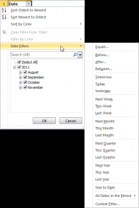
Recently, one of my viewers asked me to go into greater detail in demonstrating how the new Natural Language Date Filters work in Excel. Natural Language Filters were introduced in Excel 2007 and they are a great tool to use! Now, instead of writing complex formulas as criteria in Advanced Filters, you can simply click, “Yesterday” to see all of the records from the previous day!

Of course, you must actually have records in your data set for that date!

The Natural Language Date Filters are related, by position, to TODAY(). The TODAY() Function is a “Volatile Function” that returns the value for the current date as found in your computer systems internal clock. The result of the TODAY() Function will change each day. And so, by definition, will the result for a “Yesterday” filter!

Filter for Specific Date

There are several methods that you can use to filter for a specific date or range of dates. One method that I demonstrate in this tutorial is the “Custom Date” dialog box.

Watch Tutorial in High Definition

Follow this link to watch this Excel Tutorial in High Definition on my YouTube Channel – DannyRocksExcels

Learn About My New Extended Length Video Tutorials

I have recently released a series of extended length (90 minutes) video tutorials. They are part of my “Master Excel in Minutes” Series. Each video focuses on one topic. My first video is focused on Excel Pivot Tables. I have created Videos for Excel 2010, Excel 2007 and for Excel 2003. You also have the choice of purchasing the video for immediate downloading or shipped to you on a DVD-ROM.

Follow this link to go to the information page for my “Master Excel in Minutes” video tutorial series.

Share and Enjoy:

How to Yse Natural Language Date Filters in Excel [ 6:59 ] Play Now | Play in Popup | Download (3451)

Filed Under: Data Filters and Queries, Date Functions and Formats in Excel, Excel Training, Pivot Tables, Podcast Tips & Timesavers Tagged: Date Filters in Excel, Excel Pivot Tables, Excel Video Training, Natural Language Date Filters in Excel, Tips and Time Savers, Video lessons for Excel

Danny November 21, 2011 Leave a Comment

How to Automatically Add a Time / Date Stamp Whenever You Add or Edit a Record in Excel

VBA Code to add Time Stamp

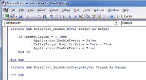
In this video tutorial, I respond to one of the most frequent requests that I get from my viewers – “How do I automatically add a ‘Time / Date Stamp’ whenever I add or edit a record in my Excel Worksheet?”

On the surface, this might appear to be a “simple” question to answer. However, I promise that you will be frustrated if you try to solve this problem by using the =NOW() Function or one or both of these Keyboard Shortcuts:

Ctrl + ; (Semi-colon) to add a Date Stamp
Ctrl + Shift + : (Colon) to add a Time Stamp

Because … NOW() is a “Volatile Function” that automatically updates to display – in all records that refer to NOW() – the current date and time. And … because, it is difficuly to automate the combination of Keyboard Shortcuts to apply a Date / Time Stamp.

So … what is the solution?

Use VBA to Create a Simple “Event Handler” Macro

Don’t get scared off! Don’t say, “I can’t write a VBA Macro!”

I PROMISE you – an Intermediate Level User of Excel – that by investing 10 minutes to watch this tutorial – that you WILL be able to automate this process to add a Time / Date Stamp whenever you add or edit a record in Excel.

I had you – the Intermediate / Early Advanced Level Excel user in mind when I created this video tutorial. I take you step-by-step through the process. I point out the potential “got’cha” steps. I am confident that I can help you to advance your skill set in Excel with this video tutorial!

Watch Tutorial in High Definition

I invite you to watch this Excel Tutorial in High Definition on my YouTube Channel – DannyRocksExcels

Visit My Online Shopping Site

I invite you to visit my new, secure online shopping site – http://shop.thecompanyrocks.com – to see all of the new products that I have created and offer for sale!

Share and Enjoy:

How to Use a VBA Macro to Automatically Create a Time - Date Stamp Whenever a Record is Changed or Added in Excel [ 9:24 ] Play Now | Play in Popup | Download (3794)

Filed Under: Date Functions and Formats in Excel, Excel Training, Excel VBA Macros, Podcast Tips & Timesavers Tagged: Event Handler VBA Macro, Excel Video Training, NOW Function in Excel, Project Exploer in VBA, Time and Date Stamp Records in Excel, VBA Macros in Excel, Video lessons for Excel

Danny July 7, 2011 1 Comment

Use Excel’s AutoFill Options and Formulas to Increment a Series of Dates

Excel AutoFill Options

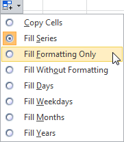
I begin this Excel Video tutorial by first, demonstrating how to use Excel’s AutoFill Options to increment a series of dates. Some of these AutoFill Options are:

Fill Weekdays Only (Monday through Friday)
Copy Formatting Only
Increment by Adding one month to the previous cell
Increment by Adding one year to the previous cell

Here’s a Tip: If you use your Right-mouse button to AutoFill a series, a menu of options will pop up automatically when you release the mouse. Try it!

Excel Functions and Formulas to Increment a Series of Dates

Two of my favorite Excel Date Functions are part of the “Analysis ToolPak” Add-in:

The EDATE() Function – returns a “serial number” for a Month that is X number of months away from the starting date.
The EOMONTH() Function – is similar to EDATE. However, it always returns the last Calendar Day of the Month that is X number of months away from the starting date.

In Excel 2007 and Excel 2010, the Analysis ToolPak Add-in is activated by default. In this video, I demonstrate how to activate it if you are using Excel 2003 or older.

Watch This Video in High Definition

Follow this link to view this video tutorial in High Definition on my YouTube Channel – DannyRocksExcels

Shop for Excel Training Resources

Shop for The 50 Best Tips for Excel 2007

I invite you to visit my secure online shopping website – http://shop.thecompanyrocks.com – to see all of the great training resources that I offer you.

Get my best-selling DVD-ROM, “The 50 Best Tips for Excel 2007” for only $39.95!

Share and Enjoy:

How to use Excel's AutoFill Options and Formulas to Increment a Series of Dates [ 11:21 ] Play Now | Play in Popup | Download (1637)

Filed Under: Date Functions and Formats in Excel, Excel Date and Time Functions, Excel Training, Podcast Tips & Timesavers Tagged: AutoFill Options, DATE() Function, EDATE Function, EOMONTH Function, Exce Date Functions, Excel Analysis Toolpak Add-in, Excel Functions, Excel Video Training, Increment Series of Dates in Excel, Learn to use AutoFill in Excel, Video lessons for Excel, WEEKDAT Function in Excel

Danny April 22, 2011 Leave a Comment

How to Use SUMIF in Excel to Total Year-to-Date Sales

One of my viewers asked for my help to use the SUMIF Function in Excel to total Year-to-Date (YTD) Sales. Generally, the SUMIF Function is very easy to set up and use. However, when you need to refer to a “date” in the criteria argument, there is a “Got’cha” step.

How to Write the Formula for Year-to-Date Sales

=SUMIF(Date, “<=”&TODAY(), Sales) Notice how the <= comparison operator is enclosed within ” ” (Quotation Marks) and I use the & (ampersand) to join the TODAY() Function. Be careful when you write this fomula. In my experience, when I try to write THIS formula in the “Functions Argument” Dialog Box, I almost always get an Error Message.

Create and Use Named Cell Ranges in SUMIF Function

As a best practice, I encourage you to create and use “Named Cell Ranges” in your formulas. This is especially helpful with the SUMIF, SUMIFS, COUNTIF, COUTIFS functions because you are usually looking inside extensive ranges of data.

Another Way to Total Year-to-Date Sales

For many years, I did not realize that there was a SUMIF Function. So, I used to create an extra column and write to formulas to compute the YTD Sales. If you do want to or need to see YTD sales in each cell, I show you how to do this by writing just one formula.

Watch Lesson in High Definition

Follow this link to view this video lesson in High Definition on my YouTube Channel – DannyRocksExcels

Download My Free Video Lessons on Pivot Tables

Click here to learn about my 24 minute video recordings “Introducing Pivot Tables.” I have two versions – One for Excel 2003 and one for Excel 2007. I am offering both of them as a “free of charge” downloadable product!

Share and Enjoy:

How to Use the SUMIF Function to Total Year to Date Sales [ 5:09 ] Play Now | Play in Popup | Download (1424)

Filed Under: Date Functions and Formats in Excel, Excel Training, Podcast Tips & Timesavers, SUMIF and SUMIFS Functions Tagged: Excel Video Training, Function Arguments Dialog Box, Named Cell in a formula, Named Cells and Ranges, SUMIF Function, TODAY() Function in Excel, Video lessons for Excel

Danny February 2, 2011 Leave a Comment

How to Use Date Functions and Date Formatting in Excel

In this lesson, I respond to two recent requests from viewers for help in Using DATE Functions in Excel and also, how to apply Custom Date Formatting. I get similar requests on a frequent basis from both viewers and clients.

Solve Problem #1

My first viewer wants help in using the DATE() Function in Excel. She wants to calculate a date that is 90 days after the starting date for a project. She encountered two problems

Initially, the DATE() Function produced and error – because she forgot to ‘nest” the YEAR(), MONTH()+9, DAY() Functions inside the DATE() Function.
She was not expecting a date to be filled in the formulas column when there was no starting date for the project – She needed to include an IF() function to perform a LOGICAL TEST – Does the Starting Date = 0, Value if TURE, ” ” (to display nothing), Value if FALSE – to perform the calculation.

Excel Custom Date Formats

Solve Problem #2

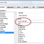
My second viewer wanted my help to ensure that the date values that he “pasted” into a range of cells were in the (Custom) format of “yyyy-mm-dd” (Year, Month, Date).

In this case, we need to take two steps:

Format the destination cells using the CUSTOM FORMAT of yyyy-mm-dd that we create.
After “Pasting” the Copied Cells, use the “Paste Options” dialog box to select – “Match Destination Formatting.”

I also demonstrate how to use the NETWORKDAYS() Function and the WORKDAY() Function – with an optional list of “Holidays” to exclude. And, finally, I show you the “pitfalls” that occur when you import a “text” file of dates that use a variety of formats. In order to perform DATE calculations, a date must be stored as a NUMBER in Excel. It must be right-aligned in the cell.

You can watch this Excel Video Lesson in High Definition, Full Screen Mode on my YouTube Channel – DannyRocksExcel – by clicking this link.

Learn to “Master Excel in Minutes – Not Months!”

Share and Enjoy:

How to Use Date Functions and Apply Date Formatting in Excel [ 12:06 ] Play Now | Play in Popup | Download (1075)

Filed Under: Date Functions and Formats in Excel, Excel Training, Podcast Tips & Timesavers Tagged: DATE() Function, DAY()Function, Excel Video Training, IF() Function, Import Text Files, MONTH()Function, NETWORKDAYS Function, Video lessons for Excel, WORKDAY Function, YEAR() Function

Danny Rocks “Training You to Excel”

Follow Danny on Social Media

Understanding Dynamic Date Functions

Improvements in Conditional Formatting

Formulas Used to Apply Conditional Formatting

Related Video

Watch this Video in High Definition

Get the Best Tips and Training for Excel

Subscribe to my Video Podcast on iTunes

Formatting Numbers to Include Text

Download this Video Podcast from iTunes

Watch Video in High Definition

Visit my Secure Online Shopping Website

What is Covered on the Video

Learn More About the “Undocumented” DATEDIF() Function

Learn How to Calculate a Calendar Year Quarter

Resources Available at The Company Rocks

Watch Video Tutorial in High Definition

Watch this Video Now

Filter for Specific Date

Watch Tutorial in High Definition

Learn About My New Extended Length Video Tutorials

Use VBA to Create a Simple “Event Handler” Macro

Watch Tutorial in High Definition

Visit My Online Shopping Site

Excel Functions and Formulas to Increment a Series of Dates

Other Functions Used in this Video Tutorial

Related Video Tutorial

Watch This Video in High Definition

Shop for Excel Training Resources

How to Write the Formula for Year-to-Date Sales

Create and Use Named Cell Ranges in SUMIF Function

Another Way to Total Year-to-Date Sales

Watch Lesson in High Definition

Download My Free Video Lessons on Pivot Tables

Solve Problem #1

Solve Problem #2

Locate My Video Tutorials by Category

Seach My Website with Keywords

Podcast Feeds

Blogroll

Blogs for Business Writing

Blogs for Excel

Blogs for Presentations

Register or Log In

Tags