How to Use a Data Validation Formula When Creating a Budget

Use Formulas in Data Validation

Use a Formula in Data Validation

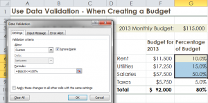
Recently, one of my viewers wanted to know which formula he could use to prevent an end-user from imputing a value that would exceed his budget. I created this video tutorial to demonstrate my response.

Use a Formula in Data Validation

I have identified Data Validation as one of the “Nine Essential Skills in Excel.” Here is one example – Using a Formula in Data Validation to prevent an input entry from exceeding a set budget amount

A Formula that Evaluates to TRUE

The “key” to understanding how use Formulas in Data Validation – When the formula answer is TRUE, the entry is accepted; When the answer to the formula is FALSE, the Error Message that you create prevents an invalid entry.

Remember, that in Data Validation, only the STOP style will prevent an invalid entry.!

Video Training Resources

9 Essential Skills for Excel 2010

9 Essential Skills for Excel 2010 Video Tutorial

I invite you to visit my secure online shopping website – http://shop.thecompanyrocks.com – to preview the many video training resources that I offer you.

Watch This Tutorial in High Definition

Follow this link to watch my Excel Tutorial in High Definition on my YouTube Channel – DannyRocksExcels

Share and Enjoy:
  • Add to favorites
  • Facebook
  • Twitter
  • Technorati
  • Print
  • email
  • Digg
  • StumbleUpon
  • del.icio.us
  • Yahoo! Buzz
  • Google Bookmarks
  • Orkut
  • SphereIt
  • Sphinn

Instructional Guide “9 Essential Excel 2010 Skills” – Download for Free

Instructional Guide "9 Essential Excel 2010 Skills"

Instructional Guide “9 Essential Excel 2010 Skills”

I want you to discover the scope of the Excel Training that I offer on my new video tutorial, “9 Essential Excel 2010 Skills.” So, I am offering the PDF of the Step-by-Step Instructional Guide that accompanies the video tutorial.

Link to The Company Rocks Free Resources Page

Click on this link to begin the download process for the Instructional Guide.

Instructions for Downloading the Free Instructional Guide

  1. Add this product to your secure shopping cart at my website.
  2. During Checkout, you can choose to either Register or Shop as a Guest
  3. You will need to provide a valid email address in order to receive the actual link to download my Instructional Guide.
  4. Even though you will be downloading this product, I had to set it up as a physical product with “Free Shipping.”
  5. Shortly after you complete the checkout process you will receive an email that contains a hyperlink to the file that you will download.
  6. You will be downloading a “zipped” file. So, once the download is completed, be sure to “unzip” this file!
  7. I created my Instructional Guide using the free Adobe Acrobat Reader.

Read the Instructional Guide and then Purchase my Video!

I am convinced that once you see the scope of the training in Excel 2010 that I offer, you will want to purchase the video tutorial. I offer my video in tow versions:

List of the “9 Essential Excel 2010 Skills”

9 Essential Skills for Excel 2010

9 Essential Skills for Excel 2010 Video Tutorial

These are the 9 Essential Skills that I have identified for my video tutorial:

  1. Entering Data Efficiently in Excel 2010
  2. Selecting Cell Ranges Efficiently in Excel 2010
  3. Creating and Using Named Cell Ranges in Excel 2010
  4. Applying Styles and Formatting to Excel 2010 Worksheets
  5. Working with Structured Data Sets in Excel 2010
  6. Working with Excel 2010 Formulas and Functions
  7. Using Paste Special Options in Excel 2010
  8. Using Data Validation in Excel 2010
  9. Using Excel 2010 “What-if” Analysis Tools

Excel 2010 Practice Files Included

When you purchase my video tutorial, you receive the same Excel 2010 Worksheets that I used while filming each of the 25 video tutorials. Using the same files as you view my videos, you will be able to practice your new skills. And, of course, you also receive the same Instructional Guide that I am offering for free!

I welcome your feedback! Please send me your comments via email – danny@thecompanyrocks.com – or by adding a comment below.

Thank you!


Share and Enjoy:
  • Add to favorites
  • Facebook
  • Twitter
  • Technorati
  • Print
  • email
  • Digg
  • StumbleUpon
  • del.icio.us
  • Yahoo! Buzz
  • Google Bookmarks
  • Orkut
  • SphereIt
  • Sphinn

How to Clear All Underlying Cell Formatting in Excel

Clear Underlying Formatting

Clear Underlying Formatting

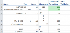
Have you ever typed data or a formula in a cell only to be surprised by the result? For example, you type in a number and then, unexpectedly,  Excel displays a Date or a Time in that cell. This happens frequently when you reuse an older Excel Worksheet of if you start working on a worksheet that a colleague or client has sent you.

Why does this happen?

Clear All Underlying Cell Formatting

In my experience, I have found that many Excel users mistakenly think that pressing the DELETE Key will “erase” the cells in the selection. No, No, No. The Delete key only erased the cell content – the data, text or formulas entered or pasted into the cell(s). The Delete key does NOT remove the Underlying Cell Formatting!

In this tutorial, I demonstrate how to remove the underlying cell formatting while leaving the cell Contents in place.

Topics Covered in this Tutorial

  • Using the Clear Formatting Command
  • Adding the Clear Command to your Quick Access Toolbar
  • Using Go To Special to Find and Select all cell that use either Conditional Formatting or Data Validation
  • Finding the Last Cell in your worksheet – you may be surprised to find a “remote cell” is NOT Blank!

View All the Resources that I Offer

I invite you to visit my secure online shopping website – http://shop.thecompanyrocks.com – to preview all of the resources that I offer.

Watch this Tutorial in High Definition

Follow this link to view this Excel Tutorial in High Definition on my YouTube Channel – DannyRocksExcels


Share and Enjoy:
  • Add to favorites
  • Facebook
  • Twitter
  • Technorati
  • Print
  • email
  • Digg
  • StumbleUpon
  • del.icio.us
  • Yahoo! Buzz
  • Google Bookmarks
  • Orkut
  • SphereIt
  • Sphinn

Use an Excel Template to Customize a Worksheet with 52 Weeks of Employee Time Cards

Template for Time Cards in Excel

Time Card Templates in Excel

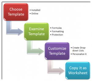
This is Part Two in my new series of Excel Tutorials where I share my best practice tips for creating 52 weeks of Employee Time Cards – for hours worked. In this segment, I focus on starting the process with an Excel Template.

Finding Templates for Time Cards

As I demonstrate in the video, there are at least two easy sources for finding a Time Card Template:

  1. Sample Templates Installed on your Computer
  2. Templates that you can preview and download from the Microsoft Office Templates Website

Examining Templates that You Download

Before you even think about duplicating the Excel Template that you just downloaded, it is important for you to take a few minutes to explore:

  • The Formulas used in the Template
  • The Formatting used in the Template – especially the formatting for Dates and Times
  • The Protection Applied (if any) to the cells or the entire worksheet

Creating Drop-down Menus for your Template

Since our premise here is that we will copy the template to 51 additional worksheets, it makes sense to use Data Validation to create a series of “drop-down menus” for Employee names and the Start Date for each week. I demonstrate how to do this in the video tutorial.

Links to Additional Video Tutorials in this Series

Additional Resources for Excel

I invite you to visit my new, secure, online shopping website – http://shop.thecompanyrocks.com – to discover the many training resources that I offer you!

Watch Tutorial in High Definition

Follow this link to watch this Excel Tutorial in High Definition on my YouTube Channel – DannyRocksExcels

Click to Watch Video Now

Share and Enjoy:
  • Add to favorites
  • Facebook
  • Twitter
  • Technorati
  • Print
  • email
  • Digg
  • StumbleUpon
  • del.icio.us
  • Yahoo! Buzz
  • Google Bookmarks
  • Orkut
  • SphereIt
  • Sphinn

How to SUM Values in One Field Based on Criteria from Multiple Fields in Excel

SUMIFS and DSUM Functions

SUMIFS and DSUM Functions

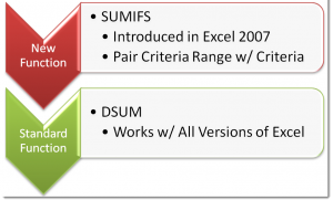
The new SUMIFS() Function was introduced in Excel 2007. With SUMIFS, you can sum the values in one field based up criteria that comes from multiple fields. This is a very valuable Function.

SUMIFS Function

The key to understanding SUMIFS, is that you “pair” a criteria range with the criteria for that range. As you watch my tutorial, the importance of this concept will become clear to you.

DSUM Function

If you are using – or need to create workbooks that are compatible with – older versions of Excel – e.g. Excel 2003, you can use the DSUM Function to achieve the same results. The DSUM belongs to the Database Functions set in Excel.

Use Named Cell Ranges in Formulas

I highly recommend that you learn how to create – and then use – named cell references in your Excel Formulas and Functions. In this tutorial, I show you how to do this. Once you have created a named cell reference, you can use the F3 Keyboard Shortcut to show a dialog box that lists all of the named Ranges that you can post into your formulas. This will save you time and help to ensure accuracy in your formulas – especially when you cop a formula to another location.

Bonus: Create Drop-down Menu with Data Validation

When using Multiple Criteria, I like to be able to select my criteria values from a drop-down list. In this lesson, I demonstrate how to do this using Data Validation in Excel.

Learn More Excel Tips

I invite you to visit my new, secure, online shopping website – http://shop.thecompanyrocks.com. Here, you can learn more about the tips on my best-selling DVD-ROM, “The 50 Best Tips for Excel 2007.”


Watch Video in High Definition

Here is the link to view this Excel Tutorial in High Definition on my YouTube Channel – DannyRocksExcels

YouTube Video

Share and Enjoy:
  • Add to favorites
  • Facebook
  • Twitter
  • Technorati
  • Print
  • email
  • Digg
  • StumbleUpon
  • del.icio.us
  • Yahoo! Buzz
  • Google Bookmarks
  • Orkut
  • SphereIt
  • Sphinn

How to Use the Offset Function Inside a VLookup in Excel

Vlookup in Excel

VLOOKUP in Excel

Each month, I get 5 to 6 emails of phone calls from viewers who who are having trouble using the VLOOKUP Function in Excel. In the majority of cases, the problem is that their Data Table is setup so that the “Key” field that they need to search in is NOT the Left-most or first field in the table. It is not always practical – nor desirable – to use “Cut and Paste” to rearrange the fields in the data set. So, what techniques can you use to fix this?

Use the OFFSET Function Inside a VLOOKUP Function

In this scenario, our IT Department sends us a daily report of the products that we sell including fields for the current cost and quantity on-hand. We use this report to generate additional reports and filters. This report gets saved automatically as an Excel 2010 Table with the name “Inventory.” The problem is, whenusing a VLOOKUP, that the first – or Left-most – field is NOT the “Key” field that we want VLOOKUP to use to search for a Match in order to return the current price or inventory for individual product.

The OFFSET() Function in Excel, makes it easy to reference a “starting field” that, in this case, is one column to the Right. This is perfect for our situation. We can continue to use our “named range” with the VLOOKUP!

Watch Video in High Definition

Follow this link to watch this tutorial in High Definition on my YouTube Channel – DannyRocksExcels

Visit My New Secure Online Shopping Website

I invite you to visit my new online shopping website at: http://shop.thecompanyrocks.com I have created new, extended length video tutorials that you can either purchase to download immediately or order them on a DVD-ROM. In addition, I have published versions of my 90 minute Pivot Tables Video Tutorials for Excel 2003, Excel 2007 and Excel 2010. So, I have the tutorials that you want for the Excel version that you are currently using!

Click to Play Excel Video Tutorial

Share and Enjoy:
  • Add to favorites
  • Facebook
  • Twitter
  • Technorati
  • Print
  • email
  • Digg
  • StumbleUpon
  • del.icio.us
  • Yahoo! Buzz
  • Google Bookmarks
  • Orkut
  • SphereIt
  • Sphinn

How to Take Advantage of the Go To Special Dialog Box Options in Excel

Go To Special Options

Go To Special Options

In my opinion, the Go To Special Options Dialog Box offers some of the most useful tools in Excel!

Why?

Because,  you must…

Select Cells Before Performing an Action on these Cells

The “key” to understanding ANY MS Office or Windows Program is… You MUST select a single cell or a range of cells BEFORE you can perform an action on them – e.g. Formatting you selection, deleting your selection, editing your selection or auditing your selection.

Tips Presented in this Video Tutorial

  • Select cells with Comments – so that you can “format” these cells to make them easier to identify.
  • Select cells that contain Constant Numeric Values – so that you can easily “spot” cells that should – bu do not – contain formulas.
  • Select cells that contain Specific Types of Formulas – e.g. Text Formulas – to “audit” your formulas.
  • Find the “Last Cell” in your worksheet – the last cell that contains EITHER content OR FORMATTING – This can be an “eye-opener!” for you.
  • Select the cells that contain Data Validation – perhaps you failed to “validate” all of the cells in a range.
  • Select the cells that contain Conditional Formatting – perhaps your did not select ALL of the cells in a Range BEFORE you applied a Conditional Formatting RULE!
  • Learn how to select the “Visible Cells Only” before performing a copy and paste operation – especially helpful when copying the “collapsed cells” for an Excel Outline.

I am positive that Excel users at ANY LEVEL will be able to pick up at least one solid tip from this Video Tutorial. Please send me your comments to let me know what you learned – or what you need clarification on.

Watch Tutorial in High Definition Mode

Follow this link to view this Excel Tutorial in High Definition / Full Screen Mode on my YouTube Channel – DannyRocksExcels

Learn About My New Extended Length Excel Video Tutorials

I have just published the first in a series of “Extended Length” – 90 Minutes – Video Tutorials, “Excel Pivot Tables to Summarize, Analyze and Present Your Data.” Follow this link to learn more about this tutorial. I have created separate versions of the tutorial for Excel 2010, 2007 and 2003.

Share and Enjoy:
  • Add to favorites
  • Facebook
  • Twitter
  • Technorati
  • Print
  • email
  • Digg
  • StumbleUpon
  • del.icio.us
  • Yahoo! Buzz
  • Google Bookmarks
  • Orkut
  • SphereIt
  • Sphinn

How to Identify and Then Delete Duplicate Records in Excel

Identify & Delete Duplicates

Identify & Delete Duplicates

It is almost inevitable that, over time, your Excel data set will contain duplicate records. This can be costly – if the duplicate records are in your mailing list. And it can also result in errors when you count and calculate data.

Three Methods to Identify and Delete Duplicate Records

In this Excel Tutorial, I demonstrate three approaches to identify duplicate records in a data set:

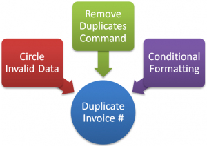
  1. Circle Invalid Data – This tool works in coordination with Data Validation.
  2. Remove Duplicates – This powerful command was introduced in Excel 2007. It does not “preview” the records to be deleted, so my advice is to use this command with a copy of your data.
  3. Conditional Formatting – Greatly improved for Excel 2007 and Excel 2010. Now, you have a menu choice to apply conditional formatting to either Duplicate or Unique Records. If you are still using Excel 2003 or earlier, I show you how to write the formula needed to use Conditional Formatting to highlight duplicate records.

Watch The Tutorial in High Definition on YouTube

Follow this link to view this Excel Tutorial in High Definition on my YouTube Channel – DannyRocksExcels

Share and Enjoy:
  • Add to favorites
  • Facebook
  • Twitter
  • Technorati
  • Print
  • email
  • Digg
  • StumbleUpon
  • del.icio.us
  • Yahoo! Buzz
  • Google Bookmarks
  • Orkut
  • SphereIt
  • Sphinn

How to Prevent Duplicate Entries in Excel with Data Validation

Formula for Data Validation

Formula for Data Validation

Over time, it is easy for duplicate entries to creep into an Excel Data Set. In this video tutorial, I show you, step-by-step, how to apply Data Validation to a range of cells so that anyone who attempts to enter a duplicate value will be prevented from doing so.

Use a “Logical Formula” for Data Validation

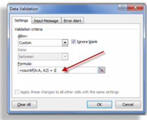
In this lesson, I show you how to “customize” the COUNTIF Function in the Data Validation Dialog Box so that it returns the value of TRUE. Logical formulas return either TRUE or FALSE. You MUST use a Logical Formula in Data Validation.

What Else is Covered in this Tutorial?

  • Use Paste Special – Validation to extend Data Validation to a wider range of cells
  • Use Find – Go to Special – Validation to highlight all cells on worksheet that contain Data Validation
  • Use Circle Invalid Entries from the Data Validation menu to automatically “draw a red circle” around existing cells that contain duplicate values
  • How to quickly remove Data Validation from a Range of Cells

Related Topic – Conditional Formatting in Excel

Another way to highlight existing cells that contain duplicate values is to use Conditional Formatting. The improvements in Excel 2007 and Excel 2010 make this “a snap” because this is now a Menu Selection! In my next tutorial, I will show you how this is done in both Excel 2003 – with the COUNTIF Function – and from the new Menu Selections introduced in Excel 2007.

Watch Tutorial in High Definition

Follow this link to my YouTube channel – DannyRocksExcels – where you can watch this tutorial in High Definition mode.

Share and Enjoy:
  • Add to favorites
  • Facebook
  • Twitter
  • Technorati
  • Print
  • email
  • Digg
  • StumbleUpon
  • del.icio.us
  • Yahoo! Buzz
  • Google Bookmarks
  • Orkut
  • SphereIt
  • Sphinn

How to Trigger a Unique List of Values Based Upon Another Drop-Down List in Excel

You can use the INDIRECT() Function in Excel to create a drop-down list of unique values that is“triggered” by the label that you select in another drop-down list. In the scenario that I use in this lesson:

  1. Create your 1st Drop-down list using Data Validation in Excel – Allow “List.” Here the named range is “Departments.”
  2. Create a 2nd Drop-down list using Data Validation. This time the “list” uses the INDIRECT Function to reference the selected label from the 1st drop-down list.

Key Concept

 The labels in my 1st drop-down list serve as “named range” references. That is why the INDIRECT Function is able to pull up the correct list of “Job Titles” in the 2nd Drop-down list. For example, a reference to the text label “Sales” in the 1st drop-down list brings up a list of the values (Job Titles) from the “Named Range” (Sales) in the 2nd Drop-down list.

If you need to learn about – or review – Data Validation in Excel, follow this link to my free Excel video lesson on this topic.

Create Named Ranges in Excel

I have found that creating and using “Named Cell Range” references makes lookup functions and formulas so much easier in Excel. Watch this video to see how I use a variety of methods to Create Named Ranges in Excel. One tip is to use the Keyboard Shortcut “Ctrl + Shift + F3” – after you first select the Label and the Values for your Named Range.

In this lesson, I also demonstrate how to visually “flag” all of the cells that do not meet the criteria for your Data Validation. I find that most people are unaware that you can do this! I think that you will find many uses for this auditing tool as you work in Excel.

Additional Resources

Follow this link to watch this video on YouTube in High Definition, Full Screen Mode.

Here is the link to view the 2nd video in this series about the INDIRECT Function in Excel.

Learn how to “Master Excel in Minutes – Not Months!” – visit my new, secure shopping site – http://shop.thecompanyrocks.com

Share and Enjoy:
  • Add to favorites
  • Facebook
  • Twitter
  • Technorati
  • Print
  • email
  • Digg
  • StumbleUpon
  • del.icio.us
  • Yahoo! Buzz
  • Google Bookmarks
  • Orkut
  • SphereIt
  • Sphinn