Archives for December 2010

Posting a Series of Tips for Access 2007

50 Best Tips for Access

Access Tips on DVD

By customer request, I am going to start posting a series of Video Lessons offering tips for using Microsoft Access 2007.

Initially, I am going to focus on showing your how to integrate Access with other Office Programs (Excel and Outlook).  Depending on the response I receive from you, my viewers, I will go deeper into the program to show you how to get the most out of a Relational Database System – MS Access.

As you can see from this beautiful cover, I have published “The 50 Best Tips for Access 2007”on DVD-ROM. This image is the “Dashboard Menu” for the DVD-ROM. You just click on the category and the DVD opens up the sub-menu for the specific lessons covered in that section.

You can learn more about the contents of my DVD-ROM by:

Thank you!

Danny Rocks

The Company Rocks

How to Use Database Functions for Excel Tables and Lists

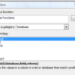
Database Functions include DSUM, DAVERAGE, DCOUNT. They are easy to use. You can use them with your Excel Tables and Lists. You use Database Functions to return the results (Sum, Average, Count, etc.) that you get from a Filter – or in this case, The Criteria.

Database Functions

Database Functions

Database Function Arguments

Each Database Function uses the same three required arguments:

  1.  
    1. Database. The Range that begins with your Data Set Labels and includes each column and each row in the database range. I prefer to use a “Named Range” for this argument.
  2. Field. The reference to the Field Label for the field that you wish to calculate (Sum, Count, Average, etc.) There are three ways to refer to this label: (Click on the cell with the label, use a column reference number (1,2,3, etc.) counting from Left to Right, type the “Label Name” inside ” ” quotation marks.
  3. Criteria. The Criteria Range that includes the Column Label for the criteria and the cells that contain the values or formulas you are using as your criteria.

It takes only a few minutes to set up your “Excel Dashboard” for the Criteria Range and your Results (e.g., the sum of the values in the field that match your criteria.) Change a value in your criteria and your results update automatically.

Filtering Data in Excel

If you use a structured data set in Excel, you probably use AutoFilters or Advanced Filters. Use Database Functions to “capture” the totals, averages, and counts of those queries.

If you need to review or learn how to apply Filters to data in Excel, watch these two lessons:

Click here to watch this video in High Definition at DannyRocksExcels on YouTube.

I invite you to shop for my DVD-ROM, “The 50 Best Tips for Excel 2007.” Click here to open a secure shopping cart.

Learn how to “Master Excel in Minutes – Not Months!”

How to Apply Criteria for Advanced Filters in Excel

You want to use Excel to do more than just store data. You want to use Excel Filters in order to get information from your data set. In order to Filter the data, you need to create and apply criteria.

Options for Filtering Data:

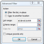
Advanced Filter Dialog Box

Advanced Filtering

  • Use the built-in AutoFilters – And, starting with Excel 2007 these include “Natural Language Filters!”
  • Use the Advanced Filter Dialog Box and your own Criteria Range – that is what I demonstrate in this lesson.

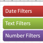
Now – since Excel 2007 – that the built-in filters include Date Filters, Text Filters and Number Filters, I do not use the Advanced Filter as much as in the past. However, there are at least two “must have” reasons to use Advanced Filters:

  1. To use “Calculated Field” criteria for your filters – e.g. to create a filter from a field that is not in your data set.
  2. To extract “Unique Records” that meet your criteria – and to copy them to another location.

I demonstrate both of these “must haves” in this video lesson.

How to Create an Advanced Filter

  1. Begin by inserting several blank rows above your Excel Data Set. These new rows will be used for your Criteria Range.
  2. Copy the Data Labels to the top row of your new Criteria Range. I like to link these with a formula – e.g. =A8 to maintain consistency with the Data Labels.
  3. Type or copy the values, comparison operators or formulas for your criteria in the row(s) below your criteria labels.
  4. Go to the Data Tab on the Ribbon and choose the Advanced Filter Command and use the Dialog Box Options.

Distinguish “OR” criteria from “AND” criteria

  • “OR” criteria use separate rows in your criteria range. You are selecting the records that match one OR more criteria.
  • “AND” criteria are written on the SAME ROW. You are filtering for records that match ALL the criteria on that row of your criteria range.

Computed Criteria in Filters

With Advanced Filters, you can use Computed Criteria for your filters. The formula must return a value that is either TRUE or FALSE. And the Label for your computed criteria CANNOT be the same as the labels in your data set.

In this lesson I show you how to filter for Invoices that have been paid – but paid “late” – after the “due date.”

Extract Unique Records with Advanced Filter

I show you how to copy the unique records – your list of customers – to a new worksheet. This is a great tip that I picked up by reading John Walkenbach’s books! Watch the video to see how this is done.

Watch My Video in High Definition

Click here to watch this video lesson in High Definition, Full Screen Mode on the DannyRocksExcels YouTube Channel.

Master Excel in Minutes Resources

I have created extended length video tutorials for Excel. I invite you to visit my online shopping website to: Learn how to “Master Excel in Minutes – Not Months!”

How to Outline an Excel Worksheet

Many Excel worksheets – e.g. Budgets and Sales Reports – can be improved by applying an Outline. With an Outline, you can switch your focus between looking at the “big picture” and examining the details. An outline is especially useful when you are presenting numbers “interactively.” For example, when you are using a Projector and Screen to present Quarterly Sales Results during a meeting.

Outline Commands
Outline Commands

If you have set up your Excel worksheet in a “hierarchical” structure – SUMs at the bottom and to the right of each category, creating an outline is simple:

Create the Outline

  • Select a single cell in the worksheet.
  • On the Data Tab of the Ribbon (Excel 2007) go to Group – Auto Outline.
  • You now see the Outline Symbols “+ and -” above each column and to the left of each row. Depending on your data, you will also see numbers that represent the “level” of Outlining available.

Examine the Formulas

When a client sends me an Excel worksheet, one of the first steps that I take is to find all of the cells that contain formulas. A quick way to do this is with the F5 Keyboard Shortcut. This opens the “Go To” Dialog Box. Choose “Special” and then select “Formulas.” Now, all of the cells that contain Formulas are highlighted. If everything is correctly organized, then I apply the “Auto Outline” command to the worksheet.

Keyboard Shortcuts

Use the Ctrl + 8 keyboard shortcut to “toggle” between Hiding and Displaying the Outline Symbols. This is a great tip to learn – you still have the Outline, but your screen looks cleaner. And … I guarantee that several people in your audience will ask you “How did you do that?”

Custom Views

During the video lesson, I also show you how and why to apply Custom Views to your Outlines. A Custom View allows you to quickly display a different perspectives of your data. Set them up in advance – it is almost like having a PowerPoint slide presentation inside your Excel worksheet outline!

You can watch this Excel video lesson in High Definition, Full Screen mode on my DannyRocksExcels YouTube channel.

Learn how to “Master Excel in Minutes – Not Months!”

I Picked Up a New Tip Today – Filtering Your Excel Data

Yesterday, I posted an Excel Video Lesson on how to Filter your data. I focused on taking advantage of the Date Filters, Text Filters, and Number Filters introduced in Excel 2007. Today, in my email inbox, I received a great tip from Chandoo – whose tag line is “Become Awesome in Excel.”

Chandoo’s Tip – which I did not know – is to Right Mouse Click on any cell in your Excel Data Set and choose Filter – Filter by Selected Cell’s Value. As Chandoo points out, this only works in Excel 2007 and higher versions. I already use this tip in Microsoft Acces. In fact it is one of the Video Tips that I share on my DVD-ROM, “The 50 Best Tips for Access 2007.” So why didn’t I know that this would work the same way in Excel 2007? Because, I needed someone to point this out to me. Thank you Chandoo!

For me, the take-away point is to continue to explore other resources to learn from other expert users. Each – e.g. Mr. Excel – Bill Jelen; Mr. Spreadsheet – John Walkenbach, etc.) – has their own perspective on Excel. Each presents a topic in a slightly different manner. Each day is an opportunity to expand my knowledge base.

I also picked up another tip from Chandoo’s post – use the Ctrl + Shift + L Keyboard Shortcut to automatically add the Filter Drop Down Buttons to your Field Header Labels. I will use this tip on a regular basis. Now, I do not have to pick up the mouse to go to the Data Tab on the Ribbon and select Filter.

If you are using Excel 2007 and higher, note that you can also use this tip (rightmouse click in a cell) to filter by the selected cell’s Icon, Font Color and Cell Background Color. Data Visualization is one of the really great improvements introduced in Excel 2007. Click here to go to my video lesson on Data Visualization.

Tip from Chandoo
Chandoo’s Tip

I recommend that you check out Chandoo’s Excel Blog by clicking on this link. You can click on the RSS Button – or go to http://feeds2.feedburner.com/PointyHairedDilbert directly to start receiving Chandoo’s Excel tips delivered automatically to your e-mail Inbox.

 
And, by the way, you can receive my new posts automatically by going to http://feeds.feedburner.com/DannyRocks which is my RSS feed on Feedburner.
 
I have now added Chandoo’s site to my Blogroll – so just click on the link whenever you visit The Company Rocks website.
 
Let me know if you have a special tip or a favorite website or blog that you want to share with our readers. Add your comment below.

How to Filter Excel Data and Save Custom Views

With an Excel data set, you rarely want to view all of the records – hundreds or thousands of records. Rather, you want to view a subset of the data – e.g. Sales of Laptop Computers in June sold by Bob. To do this, you create and apply filters. A filter is similar to a query – you are asking a question and getting the answer – information – from your data. If this is a question that you ask frequently, you can save the filter as a Custom View.

Filter Types in Excel

Filter Types

In Excel 2007, filtering has been greatly improved with the introduction of Date Filters, Text Filters and Number Filters. Now it is easy to find the sales for “last week,” or the invoices that will be due “next month,” etc. These new filter types – also available in Access 2007 – allow you get better information quicker from your data set.

Top 10 and Above Average Filters

In this lesson, I also demonstrate how to use the “Top 10” filter. You can also use the new “Above Average” and “Below Average” number filters to quickly find your best performers.

Create Custom Views

There is one “frustration” with Custom Views: If you use Tables in Excel 2007, you cannot use a Custom View. In fact, all Custom Views are disabled if you have a Table on any worksheet in your Excel Workbook.

You can learn more about filtering in Excel – click here to watch my video on Using Advanced Filters in Excel.

Want to watch this video in High Definition, Full-screen Mode? Click here to go to my DannyRocksExcels Channel on YouTube.

View my Video Podcast on iTunes. Click here to go to my iTunes Video Podcast, “Danny Rocks Tips and Timesavers.”

Learn how to “Master Excel in Minutes – Not Months!”

Learn How to Quickly Create Excel Pivot Table Reports

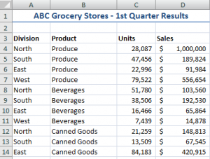
Excel Data Set

Data Set in Excel

Many people are curious about Excel Pivot Tables. They would like to learn how to create a Pivot Table, but they fear that that will take too long and be difficult to learn. 

Here’s the good news! Pivot Tables are one of the most powerful tool in Excel AND Pivot Tables are also one of the easiest Excel Techniques to learn! It sounds like a contradiction, doesn’t it? 

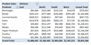
How would you like to turn this data set – with over 500 rows of data … 

into this Pivot Table Summary Report with @ six clicks of the mouse? 

Pivot Table Row & Column

Pivot Table Summary

 That’s all it takes. With a Pivot Table you turn long lists of data into summarized information that highlights the trends and patterns in your business. 

Special: Save 20% on any purchase! Use Coupon SAVE-20-PCT during Checkout! 

I can teach you how to get started on the road to mastering Excel Pivot Tables. On my DVD-ROM, “The 50 Best Tips for Excel 2007,” I have the following Pivot Table video lessons: 

  • Introducing Pivot Tables – Run time: 8:23
    • Why Use Pivot Tables?
    • How to Create a Pivot Table
    • How to Modify a Pivot Table
    • How to Update a Pivot Table
  • Grouping and Charting in Pivot Tables – Run time: 5:50
    • Grouping Pivot Table Fields by Month, Quarter and Year
    • Grouping Pivot Table Fields by Week
    • Collapsing and Expanding Pivot Table Fields
    • Creating Pivot Charts
  • Using New Pivot Table Features in Excel 2007 – Run time: 7:46
    • Base Your Pivot Table on an Excel Table
    • Adjust Pivot Table Report Layouts
    • Apply Conditional Formatting to Pivot Tables
    • Insert Blank Rows in Your Pivot Table Report
The 50 Best Tips

The 50 Best Tips Series

As you can see from the “Run times,” each lesson is focused on one Excel technique. If you don’t have a lot of time and you want to quickly learn how to create Pivot Tables, my DVD-ROM is the best place to begin. 

Here is a PDF that you can download to see the content and Run times for each of my tips: The 50 Best Tips for Excel 2007 Detailed Content Listing 

And, here is a link to my Archive of Free Pivot Table Videos  on The Company Rocks website. 

Learn how to “Quickly Create Excel Pivot Table Reports and Charts” 

Thank you! 

Danny Rocks

The 50 Best Tips for PowerPoint 2007 – Download Detailed Content Listing

50 Best Tips

Content Guide

I have created a PDF – that you can download – that details each of the learning concepts for “The 50 Best Tips for PowerPoint 2007” DVD-ROM. I also include the Run time for each video lesson so that you can schedule a lesson to fit your available time.

Follow this link to download the PDF Detailed Content List for The 50 Best Tips for PowerPoint 2007. You can print this out and also forward it to your friends and colleagues.

The PowerPoint DVD-ROM package contains two disks with over 7 hours of focused video training. I teach PowerPoint as a speaker and a trainer, NOT as a “techie.” Yes, you will learn all of the “bells and whistles” for PowerPoint, but more importantly, you will understand how, when and why to use the technique. For example, I show you the steps to take to create custom animation for your bullet points, but I also explain when you should use them and when not to.

Even if you have been using PowerPoint for many years I know that you will pick up many new tips that will make you more productive in producing your slide show and more effective when you make your presentation.

You can purchase the DVD-ROM for “The 50 Best Tips for PowerPoint 2007”right here on my website. I use a secure shopping cart. I accept all major credit cards and PayPal. I offer a variety of shipping options and ship to all countries. Your satisfaction is important to me. I guarantee my products 100%. If, for any reason, you are not happy with any of my products, I will refund your purchase price with no questions asked.

Click here to start shopping. 

If you received a feed of my post from yesterday – with a link to the PDF for the Excel Detailed Content List –  I have corrected a few errors in the original. Here is the link to the Excel PDF:

The 50 Best Tips for Excel 2007 Detailed Content Listing

The 50 Best Tips for Excel 2007 – Download Detailed Content Listing

By request, I have created a detailed content listing of each of “The 50 Best Tips for Excel 2007” available for you to download. Not only do you get a List of the 50 Best Tips, you also get details of the learning points in each tip and the Run time for each video lesson.  

Excel Tip List

Excel DVD Tips

You can download: 

If you would like to receive this detailed content listing as an Excel File, please click on this link to contact me directly. I will email you the file as an attachment. 

There are over 5 1/2 hours of focused video instruction on my DVD-ROM.The files are Shockwave Flash Files and they play in any Internet Browser (Internet Explorer, FireFox,Safari, etc.) 

As a bonus, the DVD-ROM contains the 50 Excel Workbooks that I use in the video lessons. Use these workbooks to recreate the lessons that you learn on the video. 

I invite you to visit my online store ( http://shop.thecompanyrocks.com) to purchase the DVD-ROM for “The 50 Best Tips for Excel 2007.” Click here to start shopping using my secure shopping cart. I guarantee your complete satisfaction with my products. If you are not satisfied, I will refund your purchase price with no questions asked. 

You will learn how to “Master Excel in Minutes – Not Months!”

Sincerely, 

Danny Rocks

Using the Built-in Excel Data Form to Edit, Enter and View Records

Data Form in Excel

Data Form

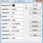
Excel has a built-in Data Form which is very useful for viewing all of the fields (up to 32 of them) associated with a single record. When you have lots of “Fields” in your “Data Set” and you do not want to do a lot of horizontal scrolling to view or edit the values in the cells, use this Data Form.

There is a limit of 32 fields when using Excel’s built-in Data Form.

Customize the Quick Access Toolbar

However, it does not appear as a Ribbon Command in Excel 2007. To use the Data Form add the Form Command to your Quick Access Toolbar (QAT) – I show you how to do this in the video.

Personally, I do not recommend the Excel Data Form for entering new records in your data set. I like to add Data Validation drop-down lists to ensure data integrity and this feature is not available in the Data Form. However, you can use Criteria to quickly find records for viewing and editing in the form.

Filtering Data with the Data Form

I give you a brief introduction to some of the new filtering options available in Excel 2007. I will cover this in greater detail in another lesson.

Subscribe to My Video Podcast on iTunes

I invite you to subscribe to my free video podcast, “Danny Rocks Tips and Timesavers” on iTunes. Click here to go directly to my iTunes podcast. I have had over 25,000 downloads since I began my podcast in June of 2010.

Watch this video in High Definition

Click here to go to my DannyRocksExcels YouTube Channel.

Watch Video Now

Master Excel in Minutes Video Training Resources

I have created a series of extended length Excel Video Training Resources. I invite you to visit my secure online shopping site to: Learn how to “Master Excel in Minutes – Not Months!”